Image features

In this chapter we will describe a set of quantitative image features together with the reference values established by the IBSI. This feature set builds upon the feature sets proposed by [Aerts2014] and [Hatt2016], which are themselves largely derived from earlier works. References to earlier work are provided whenever they could be identified.

Reference values were derived for each feature. A table of reference values contains the values that could be reliably reproduced, within a tolerance margin, for the reference data sets (see Reference data sets). Consensus on the validity of each reference value is also noted. Consensus can have four levels, depending on the number of teams that were able to produce the same value during the standardization process: weak (\(<3\) matches), moderate (\(3\) to \(5\) matches), strong (\(6\) to \(9\) matches), and very strong (\(\geq 10\) matches). If consensus on a reference value was weak or if it could not be reproduced by an absolute majority of teams, it was not considered standardized. Such features do currently not have reference values, and should not be used.

The set of features can be divided into a number of families, of which intensity-based statistical, intensity histogram-based, intensity-volume histogram-based, morphological features, local intensity, and texture matrix-based features are treated here. All texture matrices are rotationally and translationally invariant. Illumination invariance of texture matrices may be achieved by particular image post-acquisition schemes, e.g. histogram matching. None of the texture matrices are scale invariant, a property which can be useful in many (biomedical) applications. What the presented texture matrices lack, however, is directionality in combination with rotation invariance. These may be achieved by local binary patterns and steerable filters, which however fall beyond the scope of the current work. For these and other texture features, see [Depeursinge2014].

Features are calculated on the base image, as well as images transformed using wavelet or Gabor filters). To calculate features, it is assumed that an image segmentation mask exists, which identifies the voxels located within a region of interest (ROI). The ROI itself consists of two masks, an intensity mask and a morphological mask. These masks may be identical, but not necessarily so, as described in the section on Re-segmentation.

Several feature families require additional image processing steps before feature calculation. Notably intensity histogram and texture feature families require prior discretisation of intensities into grey level bins. Other feature families do not require discretisation before calculations. For more details on image processing, see Fig. 1 in the previous chapter.

Below is an overview table that summarises image processing requirements for the different feature families.

Table 2 Feature families and required image processing. For each feature family, the number of features in the document, the required input of a morphological (morph.) and/or intensity (int.) ROI mask, as well as the requirement of image discretisation (discr.) is provided. ^a The entire image volume should be available when computing local intensity features. ^b Image discretisation for the intensity-volume histogram is performed with finer discretisation than required for e.g. textural features.

		ROI mask
Feature family	count	morph.	int.	discr.
morphology	29	✔	✔	✕
local intensity	2	✕	✔ a	✕
intensity-based statistics	18	✕	✔	✕
intensity histogram	23	✕	✔	✔
intensity-volume histogram	5	✕	✔	✔ b
grey level co-occurrence matrix	25	✕	✔	✔
grey level run length matrix	16	✕	✔	✔
grey level size zone matrix	16	✕	✔	✔
grey level distance zone matrix	16	✔	✔	✔
neighbourhood grey tone difference matrix	5	✕	✔	✔
neighbouring grey level dependence matrix	17	✕	✔	✔

Though image processing parameters affect feature values, three other concepts influence feature values for many features: distance, feature aggregation and distance weighting. These are described below.

Grid distances

MPUJ

Grid distance is an important concept that is used by several feature families, particularly texture features. Grid distances can be measured in several ways. Let \(\mathbf{m}=\left(m_x,m_y,m_z\right)\) be the vector from a center voxel at \(\mathbf{k}=\left(k_x,k_y,k_z\right)\) to a neighbour voxel at \(\mathbf{k}+\mathbf{m}\). The following norms (distances) are used:

• \(\ell_1\) norm or Manhattan norm (LIFZ):

  \[\|\mathbf{m}\|_1 = |m_x| + |m_y| + |m_z|\]

• \(\ell_2\) norm or Euclidean norm (G9EV):

  \[\|\mathbf{m}\|_2 = \sqrt{m_x^2 + m_y^2 + m_z^2}\]

• \(\ell_{\infty}\) norm or Chebyshev norm (PVMT):

  \[\|\mathbf{m}\|_{\infty} = \text{max}(|m_x|,|m_y|,|m_z|)\]

An example of how the above norms differ in practice is shown in Fig. 8 .

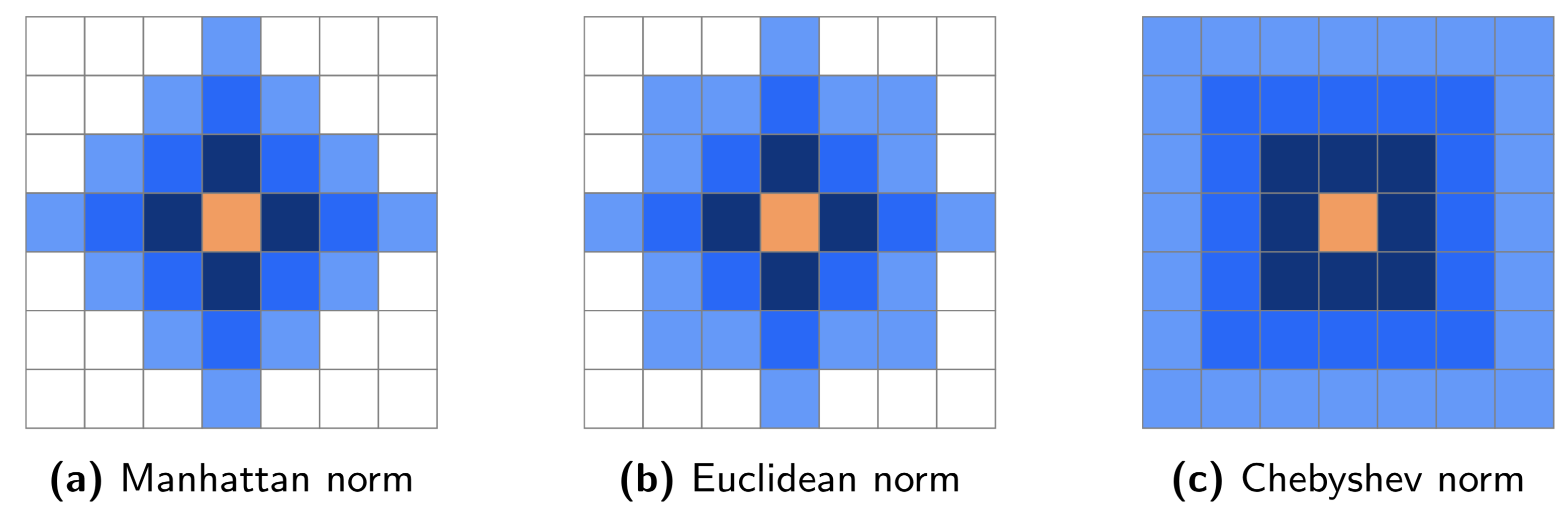
Fig. 8 Grid neighbourhoods for distances up to \(3\) according to Manhattan, Euclidean and Chebyshev norms. The orange pixel is considered the center pixel. Dark blue pixels have distance \(\delta=1\), blue pixels \(\delta\leq2\) and light blue pixels \(\delta\leq3\) for the corresponding norm.

Feature aggregation

5QB6

Features from some families may be calculated from, e.g. slices. As a consequence, multiple values for the same feature may be computed. These different values should be combined into a single value for many common purposes. This process is referred to as feature aggregation. Feature aggregation methods depend on the family, and are detailed in the family description.

Distance weighting

6CK8

Distance weighting is not a default operation for any of the texture families, but is implemented in software such as PyRadiomics [VanGriethuysen2017]. It may for example be used to put more emphasis on local intensities.

Morphological features

HCUG

Morphological features describe geometric aspects of a region of interest (ROI), such as area and volume. Morphological features are based on ROI voxel representations of the volume. Three voxel representations of the volume are conceivable:

1. The volume is represented by a collection of voxels with each voxel taking up a certain volume (LQD8).
2. The volume is represented by a voxel point set \(\mathbf{X}_{c}\) that consists of coordinates of the voxel centers (4KW8).
3. The volume is represented by a surface mesh (WRJH).

We use the second representation when the inner structure of the volume is important, and the third representation when only the outer surface structure is important. The first representation is not used outside volume approximations because it does not handle partial volume effects at the ROI edge well, and also to avoid inconsistencies in feature values introduced by mixing representations in small voxel volumes.

Mesh-based representation

A mesh-based representation of the outer surface allows consistent evaluation of the surface volume and area independent of size. Voxel-based representations lead to partial volume effects and over-estimation of the surface area. The surface of the ROI volume is translated into a triangle mesh using a meshing algorithm. While multiple meshing algorithms exist, we suggest the use of the Marching Cubes algorithm [Lorensen1987][Lewiner2003] because of its widespread availability in different programming languages and reasonable approximation of the surface area and volume [Stelldinger2007]. In practice, mesh-based feature values depend upon the meshing algorithm and small differences may occur between implementations [Limkin2019jt].

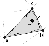
Fig. 9 Meshing algorithms draw faces and vertices to cover the ROI. One face, spanned by vertices \(\mathbf{a}\), \(\mathbf{b}\) and \(\mathbf{c}\), is highlighted. Moreover, the vertices define the three edges \(\mathbf{ab}=\mathbf{b}-\mathbf{a}\), \(\mathbf{bc}=\mathbf{c}-\mathbf{b}\) and \(\mathbf{ca}=\mathbf{a}-\mathbf{c}\). The face normal \(\mathbf{n}\) is determined using the right-hand rule, and calculated as \(\mathbf{n}=\left(\mathbf{ab} \times \mathbf{bc}\right) / \| \mathbf{ab} \times \mathbf{bc}\|\), i.e. the outer product of edge \(\mathbf{ab}\) with edge \(\mathbf{bc}\), normalised by its length.

Meshing algorithms use the ROI voxel point set \(\mathbf{X}_{c}\) to create a closed mesh. Dependent on the algorithm, a parameter is required to specify where the mesh should be drawn. A default level of 0.5 times the voxel spacing is used for marching cube algorithms. Other algorithms require a so-called isovalue, for which a value of 0.5 can be used since the ROI mask consists of \(0\) and \(1\) values, and we want to roughly draw the mesh half-way between voxel centers. Depending on implementation, algorithms may also require padding of the ROI mask with non-ROI (\(0\)) voxels to correctly estimate the mesh in places where ROI voxels would otherwise be located at the edge of the mask.

The closed mesh drawn by the meshing algorithm consists of \(N_{fc}\) triangle faces spanned by \(N_{vx}\) vertex points. An example triangle face is drawn in Fig. 9. The set of vertex points is then \(\mathbf{X}_{vx}\).

The calculation of the mesh volume requires that all faces have the same orientation of the face normal. Consistent orientation can be checked by the fact that in a regular, closed mesh, all edges are shared between exactly two faces. Given the edge spanned by vertices \(\mathbf{a}\) and \(\mathbf{b}\), the edge must be \(\mathbf{ab}=\mathbf{b}-\mathbf{a}\) for one face and \(\mathbf{ba}=\mathbf{a}-\mathbf{b}\) for the adjacent face. This ensures consistent application of the right-hand rule, and thus consistent orientation of the face normals. Algorithm implementations may return consistently orientated faces by default.

ROI morphological and intensity masks

The ROI consists of a morphological and an intensity mask. The morphological mask is used to calculate many of the morphological features and to generate the voxel point set \(\mathbf{X}_{c}\). Any holes within the morphological mask are understood to be the result of segmentation decisions, and thus to be intentional. The intensity mask is used to generate the voxel intensity set \(\mathbf{X}_{gl}\) with corresponding point set \(\mathbf{X}_{c,gl}\).

Aggregating features

By definition, morphological features are calculated in 3D (DHQ4), and not per slice.

Units of measurement

By definition, morphological features are computed using the unit of length as defined in the DICOM standard, i.e. millimeter for most medical imaging modalities.

If the unit of length is not defined by a standard, but is explicitly defined as meta data, this definition should be used. In this case, care should be taken that this definition is consistent across all data in the cohort.

If a feature value should be expressed as a different unit of length, e.g. cm instead of mm, such conversions should take place after computing the value using the standard units.

Volume (mesh)

RNU0

The mesh-based volume \(V\) is calculated from the ROI mesh as follows [Zhang2001]. A tetrahedron is formed by each face \(k\) and the origin. By placing the origin vertex of each tetrahedron at \((0,0,0)\), the signed volume of the tetrahedron is:

\[V_k = \frac{\mathbf{a}\cdot\left(\mathbf{b}\times\mathbf{c}\right)}{6}\]

Here \(\mathbf{a}\), \(\mathbf{b}\) and \(\mathbf{c}\) are the vertex points of face \(k\). Depending on the orientation of the normal, the signed volume may be positive or negative. Hence, the orientation of face normals should be consistent, e.g. all normals must be either pointing outward or inward. The volume \(V\) is then calculated by summing over the face volumes, and taking the absolute value:

\[F_{\mathit{morph.vol}} = V = \left|\sum_{k=1}^{N_{fc}}V_k\right|\]

In positron emission tomography, the volume of the ROI commonly receives a name related to the radioactive tracer, e.g. metabolically active tumour volume (MATV) for ¹⁸F-FDG.

Table 3 Reference values for the volume (mesh) feature.

data	value	tol.	consensus
dig. phantom	556	4	very strong
config. A	\(3.58 \times 10^{5}\)	\(5 \times 10^{3}\)	very strong
config. B	\(3.58 \times 10^{5}\)	\(5 \times 10^{3}\)	strong
config. C	\(3.67 \times 10^{5}\)	\(6 \times 10^{3}\)	strong
config. D	\(3.67 \times 10^{5}\)	\(6 \times 10^{3}\)	strong
config. E	\(3.67 \times 10^{5}\)	\(6 \times 10^{3}\)	strong

Volume (voxel counting)

YEKZ

In clinical practice, volumes are commonly determined by counting voxels. For volumes consisting of a large number of voxels (1000s), the differences between voxel counting and mesh-based approaches are usually negligible. However for volumes with a low number of voxels (10s to 100s), voxel counting will overestimate volume compared to the mesh-based approach. It is therefore only used as a reference feature, and not in the calculation of other morphological features.

Voxel counting volume is defined as:

\[F_{\mathit{morph.approx.vol}} = \sum_{k=1}^{N_v} V_k\]

Here \(N_v\) is the number of voxels in the morphological mask of the ROI, and \(V_k\) the volume of voxel \(k\).

Table 4 Reference values for the volume (voxel counting) feature.

data	value	tol.	consensus
dig. phantom	592	4	very strong
config. A	\(3.59 \times 10^{5}\)	\(5 \times 10^{3}\)	strong
config. B	\(3.58 \times 10^{5}\)	\(5 \times 10^{3}\)	strong
config. C	\(3.68 \times 10^{5}\)	\(6 \times 10^{3}\)	strong
config. D	\(3.68 \times 10^{5}\)	\(6 \times 10^{3}\)	strong
config. E	\(3.68 \times 10^{5}\)	\(6 \times 10^{3}\)	strong

Surface area (mesh)

C0JK

The surface area \(A\) is also calculated from the ROI mesh by summing over the triangular face surface areas [Aerts2014]. By definition, the area of face \(k\) is:

\[A_k = \frac{|\mathbf{ab} \times \mathbf{ac}|}{2}\]

As in Fig. 9, edge \(\mathbf{ab}=\mathbf{b}-\mathbf{a}\) is the vector from vertex \(\mathbf{a}\) to vertex \(\mathbf{b}\), and edge \(\mathbf{ac}=\mathbf{c}-\mathbf{a}\) the vector from vertex \(\mathbf{a}\) to vertex \(\mathbf{c}\). The total surface area \(A\) is then:

\[F_{\mathit{morph.area}} = A = \sum_{k=1}^{N_{fc}} A_k\]

Table 5 Reference values for the surface area (mesh) feature.

data	value	tol.	consensus
dig. phantom	388	3	very strong
config. A	\(3.57 \times 10^{4}\)	300	strong
config. B	\(3.37 \times 10^{4}\)	300	strong
config. C	\(3.43 \times 10^{4}\)	400	strong
config. D	\(3.43 \times 10^{4}\)	400	strong
config. E	\(3.43 \times 10^{4}\)	400	strong

Surface to volume ratio

2PR5

The surface to volume ratio is given as [Aerts2014]:

\[F_{\mathit{morph.av}} = \frac{A}{V}\]

Note that this feature is not dimensionless.

Table 6 Reference values for the surface to volume ratio feature.

data	value	tol.	consensus
dig. phantom	0.698	0.004	very strong
config. A	0.0996	0.0005	strong
config. B	0.0944	0.0005	strong
config. C	0.0934	0.0007	strong
config. D	0.0934	0.0007	strong
config. E	0.0934	0.0007	strong

Compactness 1

SKGS

Several features (compactness 1 and 2, spherical disproportion, sphericity and asphericity) quantify the deviation of the ROI volume from a representative spheroid. All these definitions can be derived from one another. As a results these features are are highly correlated and may thus be redundant. Compactness 1 [Aerts2014] is a measure for how compact, or sphere-like the volume is. It is defined as:

\[F_{\mathit{morph.comp.1}} = \frac{V}{\pi^{1/2} A^{3/2}}\]

Compactness 1 is sometimes [Aerts2014] defined using \(A^{2/3}\) instead of \(A^{3/2}\), but this does not lead to a dimensionless quantity.

Table 7 Reference values for the compactness 1 feature. An unset value (—) indicates the lack of a reference value.

data	value	tol.	consensus
dig. phantom	0.0411	0.0003	strong
config. A	0.03	0.0001	strong
config. B	0.0326	0.0001	strong
config. C	—	—	moderate
config. D	0.0326	0.0002	strong
config. E	0.0326	0.0002	strong

Compactness 2

BQWJ

Like Compactness 1, Compactness 2 [Aerts2014] quantifies how sphere-like the volume is:

\[F_{\mathit{morph.comp.2}} = 36\pi\frac{V^2}{A^3}\]

By definition \(F_{\mathit{morph.comp.1}} = 1/6\pi \left(F_{\mathit{morph.comp.2}}\right)^{1/2}\).

Table 8 Reference values for the compactness 2 feature.

data	value	tol.	consensus
dig. phantom	0.599	0.004	strong
config. A	0.319	0.001	strong
config. B	0.377	0.001	strong
config. C	0.378	0.004	strong
config. D	0.378	0.004	strong
config. E	0.378	0.004	strong

Spherical disproportion

KRCK

Spherical disproportion [Aerts2014] likewise describes how sphere-like the volume is:

\[F_{\mathit{morph.sph.dispr}} = \frac{A}{4\pi R^2} = \frac{A}{\left(36\pi V^2\right)^{1/3}}\]

By definition \(F_{\mathit{morph.sph.dispr}} = \left(F_{\mathit{morph.comp.2}}\right)^{-1/3}\).

Table 9 Reference values for the spherical disproportion feature.

data	value	tol.	consensus
dig. phantom	1.19	0.01	strong
config. A	1.46	0.01	strong
config. B	1.38	0.01	strong
config. C	1.38	0.01	strong
config. D	1.38	0.01	strong
config. E	1.38	0.01	strong

Sphericity

QCFX

Sphericity [Aerts2014] is a further measure to describe how sphere-like the volume is:

\[F_{\mathit{morph.sphericity}} = \frac{\left(36\pi V^2\right)^{1/3}}{A}\]

By definition \(F_{\mathit{morph.sphericity}} = \left(F_{\mathit{morph.comp.2}}\right)^{1/3}\).

Table 10 Reference values for the sphericity feature.

data	value	tol.	consensus
dig. phantom	0.843	0.005	very strong
config. A	0.683	0.001	strong
config. B	0.722	0.001	strong
config. C	0.723	0.003	strong
config. D	0.723	0.003	strong
config. E	0.723	0.003	strong

Asphericity

25C7

Asphericity [Apostolova2014] also describes how much the ROI deviates from a perfect sphere, with perfectly spherical volumes having an asphericity of 0. Asphericity is defined as:

\[F_{\mathit{morph.asphericity}}=\left(\frac{1}{36\pi}\frac{A^3}{V^2}\right)^{1/3}-1\]

By definition \(F_{\mathit{morph.asphericity}} = \left(F_{\mathit{morph.comp.2}}\right)^{-1/3}-1\)

Table 11 Reference values for the asphericity feature.

data	value	tol.	consensus
dig. phantom	0.186	0.001	strong
config. A	0.463	0.002	strong
config. B	0.385	0.001	moderate
config. C	0.383	0.004	strong
config. D	0.383	0.004	strong
config. E	0.383	0.004	strong

Centre of mass shift

KLMA

The distance between the ROI volume centroid and the intensity-weighted ROI volume is an abstraction of the spatial distribution of low/high intensity regions within the ROI. Let \(N_{v,m}\) be the number of voxels in the morphological mask. The ROI volume centre of mass is calculated from the morphological voxel point set \(\mathbf{X}_{c}\) as follows:

\[\overrightarrow{CoM}_{geom} = \frac{1}{N_{v,m}}\sum_{k=1}^{N_{v,m}} \vec{X}_{c,k}\]

The intensity-weighted ROI volume is based on the intensity mask. The position of each voxel centre in the intensity mask voxel set \(\mathbf{X}_{c,gl}\) is weighted by its corresponding intensity \(\mathbf{X}_{gl}\). Therefore, with \(N_{v,gl}\) the number of voxels in the intensity mask:

\[\overrightarrow{CoM}_{gl} =\frac{\sum_{k=1}^{N_{v,gl}} X_{gl,k}\vec{X}_{c,gl,k}}{\sum_{k=1}^{N_{v,gl}} X_{gl,k}}\]

The distance between the two centres of mass is then:

\[F_{\mathit{morph.com}} = ||\overrightarrow{CoM}_{geom}-\overrightarrow{CoM}_{gl}||_2\]

Table 12 Reference values for the centre of mass shift feature.

data	value	tol.	consensus
dig. phantom	0.672	0.004	very strong
config. A	52.9	28.7	strong
config. B	63.1	29.6	strong
config. C	45.6	2.8	strong
config. D	64.9	2.8	strong
config. E	68.5	2.1	moderate

Maximum 3D diameter

L0JK

The maximum 3D diameter [Aerts2014] is the distance between the two most distant vertices in the ROI mesh vertex set \(\mathbf{X}_{vx}\):

\[F_{\mathit{morph.diam}} = \text{max}\left( ||\vec{X}_{vx,k_{1}}-\vec{X}_{vx,k_{2}}||_2\right),\qquad k_{1}=1,\ldots,N\qquad k_{2}=1,\ldots,N\]

A practical way of determining the maximum 3D diameter is to first construct the convex hull of the ROI mesh. The convex hull vertex set \(\mathbf{X}_{vx,convex}\) is guaranteed to contain the two most distant vertices of \(\mathbf{X}_{vx}\). This significantly reduces the computational cost of calculating distances between all vertices. Despite the remaining \(O(n^2)\) cost of calculating distances between different vertices, \(\mathbf{X}_{vx,convex}\) is usually considerably smaller in size than \(\mathbf{X}_{vx}\). Moreover, the convex hull is later used for the calculation of other morphological features (Volume density (convex hull) - Area density (convex hull)).

Table 13 Reference values for the maximum 3D diameter feature.

data	value	tol.	consensus
dig. phantom	13.1	0.1	strong
config. A	125	1	strong
config. B	125	1	strong
config. C	125	1	strong
config. D	125	1	strong
config. E	125	1	strong

Major axis length

TDIC

Principal component analysis (PCA) can be used to determine the main orientation of the ROI [Solomon2011]. On a three dimensional object, PCA yields three orthogonal eigenvectors \(\left\lbrace e_1,e_2,e_3\right\rbrace\) and three eigenvalues \(\left( \lambda_1, \lambda_2, \lambda_3\right)\). These eigenvalues and eigenvectors geometrically describe a triaxial ellipsoid. The three eigenvectors determine the orientation of the ellipsoid, whereas the eigenvalues provide a measure of how far the ellipsoid extends along each eigenvector. Several features make use of principal component analysis, namely major, minor and least axis length, elongation, flatness, and approximate enclosing ellipsoid volume and area density.

The eigenvalues can be ordered so that \(\lambda_{\mathit{major}} \geq \lambda_{\mathit{minor}}\geq \lambda_{\mathit{least}}\) correspond to the major, minor and least axes of the ellipsoid respectively. The semi-axes lengths \(a\), \(b\) and \(c\) for the major, minor and least axes are then \(2\sqrt{\lambda_{\mathit{major}}}\), \(2\sqrt{\lambda_{\mathit{minor}}}\) and \(2\sqrt{\lambda_{\mathit{least}}}\) respectively. The major axis length is twice the semi-axis length \(a\), determined using the largest eigenvalue obtained by PCA on the point set of voxel centers \(\mathbf{X}_{c}\) [Heiberger2015]:

\[F_{\mathit{morph.pca.major}} = 2a = 4\sqrt{\lambda_{\mathit{major}}}\]

Table 14 Reference values for the major axis length feature.

data	value	tol.	consensus
dig. phantom	11.4	0.1	very strong
config. A	92.7	0.4	very strong
config. B	92.6	0.4	strong
config. C	93.3	0.5	strong
config. D	93.3	0.5	strong
config. E	93.3	0.5	strong

Minor axis length

P9VJ

The minor axis length of the ROI provides a measure of how far the volume extends along the second largest axis. The minor axis length is twice the semi-axis length \(b\), determined using the second largest eigenvalue obtained by PCA, as described in Section Major axis length.

\[F_{\mathit{morph.pca.minor}}= 2b =4\sqrt{\lambda_{\mathit{minor}}}\]

Table 15 Reference values for the minor axis length feature.

data	value	tol.	consensus
dig. phantom	9.31	0.06	very strong
config. A	81.5	0.4	very strong
config. B	81.3	0.4	strong
config. C	82	0.5	strong
config. D	82	0.5	strong
config. E	82	0.5	strong

Least axis length

7J51

The least axis is the axis along which the object is least extended. The least axis length is twice the semi-axis length \(c\), determined using the smallest eigenvalue obtained by PCA, as described in Section Major axis length.

\[F_{\mathit{morph.pca.least}}= 2c =4\sqrt{\lambda_{\mathit{least}}}\]

Table 16 Reference values for the least axis length feature.

data	value	tol.	consensus
dig. phantom	8.54	0.05	very strong
config. A	70.1	0.3	strong
config. B	70.2	0.3	strong
config. C	70.9	0.4	strong
config. D	70.9	0.4	strong
config. E	70.9	0.4	strong

Elongation

Q3CK

The ratio of the major and minor principal axis lengths could be viewed as the extent to which a volume is longer than it is wide, i.e. is eccentric. For computational reasons, we express elongation as an inverse ratio. 1 is thus completely non-elongated, e.g. a sphere, and smaller values express greater elongation of the ROI volume.

\[F_{\mathit{morph.pca.elongation}} =\sqrt{\frac{\lambda_{minor}}{\lambda_{major}}}\]

Table 17 Reference values for the elongation feature.

data	value	tol.	consensus
dig. phantom	0.816	0.005	very strong
config. A	0.879	0.001	strong
config. B	0.878	0.001	strong
config. C	0.879	0.001	strong
config. D	0.879	0.001	strong
config. E	0.879	0.001	strong

Flatness

N17B

The ratio of the major and least axis lengths could be viewed as the extent to which a volume is flat relative to its length. For computational reasons, we express flatness as an inverse ratio. 1 is thus completely non-flat, e.g. a sphere, and smaller values express objects which are increasingly flatter.

\[F_{\mathit{morph.pca.flatness}} = \sqrt{\frac{\lambda_{least}}{\lambda_{major}}}\]

Table 18 Reference values for the flatness feature.

data	value	tol.	consensus
dig. phantom	0.749	0.005	very strong
config. A	0.756	0.001	strong
config. B	0.758	0.001	strong
config. C	0.76	0.001	strong
config. D	0.76	0.001	strong
config. E	0.76	0.001	strong

Volume density (axis-aligned bounding box)

PBX1

Volume density is the fraction of the ROI volume and a comparison volume. Here the comparison volume is that of the axis-aligned bounding box (AABB) of the ROI mesh vertex set \(\mathbf{X}_{vx}\) or the ROI mesh convex hull vertex set \(\mathbf{X}_{vx,convex}\). Both vertex sets generate an identical bounding box, which is the smallest box enclosing the vertex set, and aligned with the axes of the reference frame.

\[F_{\mathit{morph.v.dens.aabb}} = \frac{V}{V_{\mathit{aabb}}}\]

This feature is also called extent [ElNaqa2009][Solomon2011].

Table 19 Reference values for the volume density (AABB) feature.

data	value	tol.	consensus
dig. phantom	0.869	0.005	strong
config. A	0.486	0.003	strong
config. B	0.477	0.003	strong
config. C	0.478	0.003	strong
config. D	0.478	0.003	strong
config. E	0.478	0.003	strong

Area density (axis-aligned bounding box)

R59B

Conceptually similar to the volume density (AABB) feature, area density considers the ratio of the ROI surface area and the surface area \(A_{aabb}\) of the axis-aligned bounding box enclosing the ROI mesh vertex set \(\mathbf{X}_{vx}\) [VanDijk2016]. The bounding box is identical to the one used for computing the volume density (AABB) feature. Thus:

\[F_{\mathit{morph.a.dens.aabb}} = \frac{A}{A_{aabb}}\]

Table 20 Reference values for the area density (AABB) feature.

data	value	tol.	consensus
dig. phantom	0.866	0.005	strong
config. A	0.725	0.003	strong
config. B	0.678	0.003	strong
config. C	0.678	0.003	strong
config. D	0.678	0.003	strong
config. E	0.678	0.003	strong

Volume density (oriented minimum bounding box)

ZH1A

Note: This feature currently has no reference values and should not be used.

The volume of an axis-aligned bounding box is generally not the smallest obtainable volume enclosing the ROI. By orienting the box along a different set of axes, a smaller enclosing volume may be attainable. The oriented minimum bounding box (OMBB) of the ROI mesh vertex set \(\mathbf{X}_{vx}\) or \(\mathbf{X}_{vx,convex}\) encloses the vertex set and has the smallest possible volume. A 3D rotating callipers technique was devised by [ORourke1985] to derive the oriented minimum bounding box. Due to computational complexity of this technique, the oriented minimum bounding box is commonly approximated at lower complexity, see e.g. [Barequet2001] and [Chan2001]. Thus:

\[F_{\mathit{morph.v.dens.ombb}} = \frac{V}{V_{ombb}}\]

Here \(V_{ombb}\) is the volume of the oriented minimum bounding box.

Area density (oriented minimum bounding box)

IQYR

Note: This feature currently has no reference values and should not be used.

The area density (OMBB) is estimated as:

\[F_{\mathit{morph.a.dens.ombb}} = \frac{A}{A_{ombb}}\]

Here \(A_{ombb}\) is the surface area of the same bounding box as calculated for the volume density (OMBB) feature.

Volume density (approximate enclosing ellipsoid)

6BDE

The eigenvectors and eigenvalues from PCA of the ROI voxel center point set \(\mathbf{X}_{c}\) can be used to describe an ellipsoid approximating the point cloud [Mazurowski2016], i.e. the approximate enclosing ellipsoid (AEE). The volume of this ellipsoid is \(V_{\mathit{aee}}=4 \pi\,a\,b\,c /3\), with \(a\), \(b\), and \(c\) being the lengths of the ellipsoid’s semi-principal axes, see Section Major axis length. The volume density (AEE) is then:

\[F_{\mathit{morph.v.dens.aee}} = \frac{3V}{4\pi abc}\]

Table 21 Reference values for the volume density (AEE) feature.

data	value	tol.	consensus
dig. phantom	1.17	0.01	moderate
config. A	1.29	0.01	strong
config. B	1.29	0.01	strong
config. C	1.29	0.01	moderate
config. D	1.29	0.01	moderate
config. E	1.29	0.01	strong

Area density (approximate enclosing ellipsoid)

RDD2

The surface area of an ellipsoid can generally not be evaluated in an elementary form. However, it is possible to approximate the surface using an infinite series. We use the same semi-principal axes as for the volume density (AEE) feature and define:

\[A_{\mathit{aee}}\left(a,b,c\right)=4\pi\,a\,b\sum_{\nu=0}^{\infty}\frac{\left(\alpha\,\beta\right)^{\nu}}{1-4\nu^2}P_{\nu}\left(\frac{\alpha^2+\beta^2}{2\alpha\beta}\right)\]

Here \(\alpha=\sqrt{1-b^2/a^2}\) and \(\beta=\sqrt{1-c^2/a^2}\) are eccentricities of the ellipsoid and \(P_{\nu}\) is the Legendre polynomial function for degree \(\nu\). The Legendre polynomial series, though infinite, converges, and approximation may be stopped early when the incremental gains in precision become limited. By default, we stop the series after \(\nu=20\).

The area density (AEE) is then approximated as:

\[F_{\mathit{morph.a.dens.aee}} = \frac{A}{A_{\mathit{aee}}}\]

Table 22 Reference values for the area density (AEE) feature.

data	value	tol.	consensus
dig. phantom	1.36	0.01	moderate
config. A	1.71	0.01	moderate
config. B	1.62	0.01	moderate
config. C	1.62	0.01	moderate
config. D	1.62	0.01	moderate
config. E	1.62	0.01	strong

Volume density (minimum volume enclosing ellipsoid)

SWZ1

Note: This feature currently has no reference values and should not be used.

The minimum volume enclosing ellipsoid (MVEE), unlike the approximate enclosing ellipsoid, is the smallest ellipsoid that encloses the ROI. Direct computation of the MVEE is usually unfeasible, and is therefore approximated. Various approximation algorithms have been described, e.g. [Todd2007][Ahipasaoglu2015], which are usually elaborations on Khachiyan’s barycentric coordinate descent method [Khachiyan1996].

The MVEE encloses the ROI mesh vertex set \(\mathbf{X}_{vx}\), and by definition \(\mathbf{X}_{vx,convex}\) as well. Use of the convex mesh set \(\mathbf{X}_{vx,convex}\) is recommended due to its sparsity compared to the full vertex set. The volume of the MVEE is defined by its semi-axes lengths \(V_{\mathit{mvee}}=4 \pi\,a\,b\,c /3\). Then:

\[F_{\mathit{morph.v.dens.mvee}} = \frac{V}{V_{\mathit{mvee}}}\]

For Khachiyan’s barycentric coordinate descent-based methods we use a default tolerance \(\tau=0.001\) as stopping criterion.

Area density (minimum volume enclosing ellipsoid)

BRI8

Note: This feature currently has no reference values and should not be used.

The surface area of an ellipsoid does not have a general elementary form, but should be approximated as noted in Section Area density (approximate enclosing ellipsoid). Let the approximated surface area of the MVEE be \(A_{\mathit{mvee}}\). Then:

\[F_{\mathit{morph.a.dens.mvee}} = \frac{A}{A_{\mathit{mvee}}}\]

Volume density (convex hull)

R3ER

The convex hull encloses ROI mesh vertex set \(\mathbf{X}_{vx}\) and consists of the vertex set \(\mathbf{X}_{vx,convex}\) and corresponding faces, see section Maximum 3D diameter. The volume of the ROI mesh convex hull set \(V_{convex}\) is computed in the same way as that of the volume (mesh) feature (Volume (mesh)). The volume density can then be calculated as follows:

\[F_{\mathit{morph.v.dens.conv.hull}} = \frac{V}{V_{convex}}\]

This feature is also called solidity [ElNaqa2009][Solomon2011].

Table 23 Reference values for the volume density (convex hull) feature.

data	value	tol.	consensus
dig. phantom	0.961	0.006	strong
config. A	0.827	0.001	moderate
config. B	0.829	0.001	moderate
config. C	0.834	0.002	moderate
config. D	0.834	0.002	moderate
config. E	0.834	0.002	moderate

Area density (convex hull)

7T7F

The area of the convex hull \(A_{convex}\) is the sum of the areas of the faces of the convex hull, and is computed in the same way as the surface area (mesh) feature (Surface area (mesh) section). The convex hull is identical to the one used in the volume density (convex hull) feature. Then:

\[F_{\mathit{morph.a.dens.conv.hull}} = \frac{A}{A_{convex}}\]

Table 24 Reference values for the area density (convex hull) feature.

data	value	tol.	consensus
dig. phantom	1.03	0.01	strong
config. A	1.18	0.01	moderate
config. B	1.12	0.01	moderate
config. C	1.13	0.01	moderate
config. D	1.13	0.01	moderate
config. E	1.13	0.01	moderate

Integrated intensity

99N0

Integrated intensity is the average intensity in the ROI, multiplied by the volume. In the context of ¹⁸F-FDG-PET, this feature is often called total lesion glycolysis [Vaidya2012]. Thus:

\[F_{\mathit{morph.integ.int}}=V\;\frac{1}{N_{v,gl}}\sum_{k=1}^{N_{v,gl}} X_{gl,k}\]

\(N_{v,gl}\) is the number of voxels in the ROI intensity mask.

Table 25 Reference values for the integrated intensity feature.

data	value	tol.	consensus
dig. phantom	\(1.2 \times 10^{3}\)	10	moderate
config. A	\(4.81 \times 10^{6}\)	\(3.2 \times 10^{5}\)	strong
config. B	\(4.12 \times 10^{6}\)	\(3.2 \times 10^{5}\)	strong
config. C	\(-1.8 \times 10^{7}\)	\(1.4 \times 10^{6}\)	strong
config. D	\(-8.64 \times 10^{6}\)	\(1.56 \times 10^{6}\)	strong
config. E	\(-8.31 \times 10^{6}\)	\(1.6 \times 10^{6}\)	strong

Moran’s I index

N365

Moran’s I index is an indicator of spatial autocorrelation [Moran1950][Dale2002]. It is defined as:

\[F_{\mathit{morph.moran.i}} = \frac{N_{v,gl}}{\sum_{k_{1}=1}^{N_{v,gl}} \sum_{k_{2}=1}^{N_{v,gl}}w_{k_{1}k_{2}}} \frac{\sum_{k_{1}=1}^{N_{v,gl}}\sum_{k_{2}=1}^{N_{v,gl}} w_{k_{1}k_{2}}\left(X_{gl,k_{1}}-\mu \right) \left( X_{gl,k_{2}}-\mu \right)} {\sum_{k=1}^{N_{v,gl}} \left(X_{gl,k}-\mu \right)^2},\qquad k_{1}\neq k_{2}\]

As before \(N_{v,gl}\) is the number of voxels in the ROI intensity mask, \(\mu\) is the mean of \(\mathbf{X}_{gl}\) and \(w_{k_{1}k_{2}}\) is a weight factor, equal to the inverse Euclidean distance between voxels \(k_{1}\) and \(k_{2}\) of the point set \(\mathbf{X}_{c,gl}\) of the ROI intensity mask [DaSilva2008]. Values of Moran’s I close to 1.0, 0.0 and -1.0 indicate high spatial autocorrelation, no spatial autocorrelation and high spatial anti-autocorrelation, respectively.

Note that for an ROI containing many voxels, calculating Moran’s I index may be computationally expensive due to \(O(n^2)\) behaviour. Approximation by repeated subsampling of the ROI may be required to make the calculation tractable, at the cost of accuracy.

Table 26 Reference values for the Moran’s I index feature.

data	value	tol.	consensus
dig. phantom	0.0397	0.0003	strong
config. A	0.0322	0.0002	moderate
config. B	0.0329	0.0001	moderate
config. C	0.0824	0.0003	moderate
config. D	0.0622	0.0013	moderate
config. E	0.0596	0.0014	moderate

Geary’s C measure

NPT7

Geary’s C measure assesses spatial autocorrelation, similar to Moran’s I index [Geary1954][Dale2002]. In contrast to Moran’s I index, Geary’s C measure directly assesses intensity differences between voxels and is more sensitive to local spatial autocorrelation. This measure is defined as:

\[F_{\mathit{morph.geary.c}} = \frac{N_{v,gl}-1}{2\sum_{k_{1}=1}^{N_{v,gl}} \sum_{k_{2}=1}^{N_{v,gl}}w_{k_{1}k_{2}}} \frac{\sum_{k_{1}=1}^{N_{v,gl}}\sum_{k_{2}=1}^{N_{v,gl}} w_{k_{1}k_{2}}\left(X_{gl,k_{1}}-X_{gl,k_{2}} \right)^2} {\sum_{k=1}^{N_{v,gl}} \left(X_{gl,k}-\mu \right)^2},\qquad k_{1}\neq k_{2}\]

As with Moran’s I, \(N_{v,gl}\) is the number of voxels in the ROI intensity mask, \(\mu\) is the mean of \(\mathbf{X}_{gl}\) and \(w_{k_{1}k_{2}}\) is a weight factor, equal to the inverse Euclidean distance between voxels \(k_{1}\) and \(k_{2}\) of the ROI voxel point set \(\mathbf{X}_{c,gl}\) [DaSilva2008].

Just as Moran’s I, Geary’s C measure exhibits \(O(n^2)\) behaviour and an approximation scheme may be required to make calculation feasible for large ROIs.

Table 27 Reference values for the Geary’s C measure feature.

data	value	tol.	consensus
dig. phantom	0.974	0.006	strong
config. A	0.863	0.001	moderate
config. B	0.862	0.001	moderate
config. C	0.846	0.001	moderate
config. D	0.851	0.001	moderate
config. E	0.853	0.001	moderate

Local intensity features

9ST6

Voxel intensities within a defined neighbourhood around a center voxel are used to compute local intensity features. Unlike many other feature sets, local features do not draw solely on intensities within the ROI. While only voxels within the ROI intensity map can be used as a center voxel, the local neighbourhood draws upon all voxels regardless of being in an ROI.

Aggregating features

By definition, local intensity features are calculated in 3D (DHQ4), and not per slice.

Local intensity peak

VJGA

The local intensity peak was originally devised for reducing variance in determining standardised uptake values [Wahl2009]. It is defined as the mean intensity in a 1 cm³ spherical volume (in world coordinates), which is centered on the voxel with the maximum intensity level in the ROI intensity mask [Frings2014].

To calculate \(F_{\mathit{loc.peak.local}}\), we first select all the voxels with centers within a radius \(r=\left(\frac{3}{4 \pi}\right)^{1/3} \approx 0.62\) cm of the center of the maximum intensity voxel. Subsequently, the mean intensity of the selected voxels, including the center voxel, are calculated.

In case the maximum intensity is found in multiple voxels within the ROI, local intensity peak is calculated for each of these voxels, and the highest local intensity peak is chosen.

Table 28 Reference values for the local intensity peak feature.

data	value	tol.	consensus
dig. phantom	2.6	—	strong
config. A	\(-\)277	10	moderate
config. B	178	10	moderate
config. C	169	10	moderate
config. D	201	10	strong
config. E	181	13	moderate

Global intensity peak

0F91

The global intensity peak feature \(F_{\mathit{loc.peak.global}}\) is similar to the local intensity peak [Frings2014]. However, instead of calculating the mean intensity for the voxel(s) with the maximum intensity, the mean intensity is calculated within a 1 cm³ neighbourhood for every voxel in the ROI intensity mask. The highest intensity peak value is then selected.

Calculation of the global intensity peak feature may be accelerated by construction and application of an appropriate spatial spherical mean convolution filter, due to the convolution theorem. In this case one would first construct an empty 3D filter that will fit a 1 cm³ sphere. Within this context, the filter voxels may be represented by a point set, akin to \(\mathbf{X}_{c}\) in Morphological features. Euclidean distances in world spacing between the central voxel of the filter and every remaining voxel are computed. If this distance lies within radius \(r=\left(\frac{3}{4 \pi}\right)^{1/3} \approx 0.62\) the corresponding voxel receives a label \(1\), and \(0\) otherwise. Subsequent summation of the voxel labels yields \(N_s\), the number of voxels within the 1 cm³ sphere. The filter then becomes a spherical mean filter by dividing the labels by \(N_s\).

Table 29 Reference values for the global intensity peak feature.

data	value	tol.	consensus
dig. phantom	3.1	—	strong
config. A	189	5	moderate
config. B	178	5	moderate
config. C	180	5	moderate
config. D	201	5	moderate
config. E	181	5	moderate

Intensity-based statistical features

UHIW

The intensity-based statistical features describe how intensities within the region of interest (ROI) are distributed. The features in this set do not require discretisation, and may be used to describe a continuous intensity distribution. Intensity-based statistical features are not meaningful if the intensity scale is arbitrary.

The set of intensities of the \(N_v\) voxels included in the ROI intensity mask is denoted as \(\mathbf{X}_{gl}=\left\lbrace X_{gl,1},X_{gl,2},\ldots,X_{gl,N_v}\right\rbrace\).

Aggregating features

We recommend calculating intensity-based statistical features using the 3D volume (DHQ4). An approach that computes intensity-based statistical features per slice and subsequently averages them (3IDG) is not recommended.

Mean intensity

Q4LE

The mean intensity of \(\mathbf{X}_{gl}\) is calculated as:

\[F_{\mathit{stat.mean}} = \frac{1}{N_v}\sum_{k=1}^{N_v} X_{gl,k}\]

Table 30 Reference values for the mean feature.

data	value	tol.	consensus
dig. phantom	2.15	—	very strong
config. A	13.4	1.1	very strong
config. B	11.5	1.1	strong
config. C	\(-\)49	2.9	very strong
config. D	\(-\)23.5	3.9	strong
config. E	\(-\)22.6	4.1	strong

Intensity variance

ECT3

The intensity variance of \(\mathbf{X}_{gl}\) is defined as:

\[F_{\mathit{stat.var}} = \frac{1}{N_v}\sum_{k=1}^{N_v} \left( X_{gl,k}-\mu \right)^2\]

Note that we do not apply a bias correction when computing the variance.

Table 31 Reference values for the variance feature.

data	value	tol.	consensus
dig. phantom	3.05	—	very strong
config. A	\(1.42 \times 10^{4}\)	400	very strong
config. B	\(1.44 \times 10^{4}\)	400	very strong
config. C	\(5.06 \times 10^{4}\)	\(1.4 \times 10^{3}\)	strong
config. D	\(3.28 \times 10^{4}\)	\(2.1 \times 10^{3}\)	strong
config. E	\(3.51 \times 10^{4}\)	\(2.2 \times 10^{3}\)	strong

Intensity skewness

KE2A

The skewness of the intensity distribution of \(\mathbf{X}_{gl}\) is defined as:

\[F_{\mathit{stat.skew}} = \frac{\frac{1}{N_v}\sum_{k=1}^{N_v} \left( X_{gl,k}-\mu \right) ^3}{\left(\frac{1}{N_v}\sum_{k=1}^{N_v} \left( X_{gl,k}-\mu \right)^2\right)^{3/2}}\]

Here \(\mu=F_{\mathit{stat.mean}}\). If the intensity variance \(F_{\mathit{stat.var}} = 0\), \(F_{\mathit{stat.skew}}=0\).

Table 32 Reference values for the skewness feature.

data	value	tol.	consensus
dig. phantom	1.08	—	very strong
config. A	\(-\)2.47	0.05	very strong
config. B	\(-\)2.49	0.05	very strong
config. C	\(-\)2.14	0.05	very strong
config. D	\(-\)2.28	0.06	strong
config. E	\(-\)2.3	0.07	strong

(Excess) intensity kurtosis

IPH6

Kurtosis, or technically excess kurtosis, is a measure of peakedness in the intensity distribution \(\mathbf{X}_{gl}\):

\[F_{\mathit{stat.kurt}} = \frac{\frac{1}{N_v}\sum_{k=1}^{N_v} \left( X_{gl,k}-\mu \right) ^4}{\left(\frac{1}{N_v}\sum_{k=1}^{N_v} \left( X_{gl,k}-\mu \right)^2\right)^{2}} -3\]

Here \(\mu=F_{\mathit{stat.mean}}\). Note that kurtosis is corrected by a Fisher correction of -3 to center it on 0 for normal distributions. If the intensity variance \(F_{\mathit{stat.var}} = 0\), \(F_{\mathit{stat.kurt}}=0\).

Table 33 Reference values for the (excess) kurtosis feature.

data	value	tol.	consensus
dig. phantom	\(-\)0.355	—	very strong
config. A	5.96	0.24	very strong
config. B	5.93	0.24	very strong
config. C	3.53	0.23	very strong
config. D	4.35	0.32	strong
config. E	4.44	0.33	strong

Median intensity

Y12H

The median intensity \(F_{\mathit{stat.median}}\) is the sample median of \(\mathbf{X}_{gl}\).

Table 34 Reference values for the median feature.

data	value	tol.	consensus
dig. phantom	1	—	very strong
config. A	46	0.3	very strong
config. B	45	0.3	strong
config. C	40	0.4	strong
config. D	42	0.4	strong
config. E	43	0.5	strong

Minimum intensity

1GSF

The minimum intensity is equal to the lowest intensity present in \(\mathbf{X}_{gl}\), i.e:

\[F_{\mathit{stat.min}} = \text{min}(\mathbf{X}_{gl})\]

Table 35 Reference values for the minimum feature.

data	value	tol.	consensus
dig. phantom	1	—	very strong
config. A	\(-\)500	—	very strong
config. B	\(-\)500	—	very strong
config. C	\(-\)939	4	strong
config. D	\(-\)724	12	strong
config. E	\(-\)743	13	strong

10^th intensity percentile

QG58

\(P_{10}\) is the 10^th percentile of \(\mathbf{X}_{gl}\). \(P_{10}\) is a more robust alternative to the minimum intensity.

Table 36 Reference values for the 10th percentile feature.

data	value	tol.	consensus
dig. phantom	1	—	very strong
config. A	\(-\)129	8	strong
config. B	\(-\)136	8	strong
config. C	\(-\)424	14	very strong
config. D	\(-\)304	20	strong
config. E	\(-\)310	21	strong

90^th intensity percentile

8DWT

\(P_{90}\) is the 90^th percentile of \(\mathbf{X}_{gl}\). \(P_{90}\) is a more robust alternative to the maximum intensity.

Table 37 Reference values for the 90th percentile feature.

data	value	tol.	consensus
dig. phantom	4	—	very strong
config. A	95	—	strong
config. B	91	—	strong
config. C	86	0.1	strong
config. D	86	0.1	strong
config. E	93	0.2	strong

Note that the 90:sup:`th` intensity percentile obtained for the digital phantom may differ from the above reference value depending on the software implementation used to compute it. For example, some implementations were found to produce a value of 4.2 instead of 4.

Maximum intensity

84IY

The maximum intensity is equal to the highest intensity present in \(\mathbf{X}_{gl}\), i.e:

\[F_{\mathit{stat.max}} = \text{max}(\mathbf{X}_{gl})\]

Table 38 Reference values for the maximum feature.

data	value	tol.	consensus
dig. phantom	6	—	very strong
config. A	377	9	very strong
config. B	391	9	strong
config. C	393	10	very strong
config. D	521	22	strong
config. E	345	9	strong

Intensity interquartile range

SALO

The interquartile range (IQR) of \(\mathbf{X}_{gl}\) is defined as:

\[F_{\mathit{stat.iqr}} = P_{75}-P_{25}\]

\(P_{25}\) and \(P_{75}\) are the 25^th and 75^th percentiles of \(\mathbf{X}_{gl}\), respectively.

Table 39 Reference values for the interquartile range feature.

data	value	tol.	consensus
dig. phantom	3	—	very strong
config. A	56	0.5	very strong
config. B	52	0.5	strong
config. C	67	4.9	very strong
config. D	57	4.1	strong
config. E	62	3.5	strong

Intensity range

2OJQ

The intensity range is defined as:

\[F_{\mathit{stat.range}} = \text{max}(\mathbf{X}_{gl}) - \text{min}(\mathbf{X}_{gl})\]

Table 40 Reference values for the range feature.

data	value	tol.	consensus
dig. phantom	5	—	very strong
config. A	877	9	very strong
config. B	891	9	strong
config. C	\(1.33 \times 10^{3}\)	20	strong
config. D	\(1.24 \times 10^{3}\)	40	strong
config. E	\(1.09 \times 10^{3}\)	30	strong

Intensity-based mean absolute deviation

4FUA

Mean absolute deviation is a measure of dispersion from the mean of \(\mathbf{X}_{gl}\):

\[F_{\mathit{stat.mad}} = \frac{1}{N_v}\sum_{k=1}^{N_v} \left|X_{gl,k}-\mu\right|\]

Here \(\mu=F_{\mathit{stat.mean}}\).

Table 41 Reference values for the mean absolute deviation feature.

data	value	tol.	consensus
dig. phantom	1.55	—	very strong
config. A	73.6	1.4	very strong
config. B	74.4	1.4	strong
config. C	158	4	very strong
config. D	123	6	strong
config. E	125	6	strong

Intensity-based robust mean absolute deviation

1128

The intensity-based mean absolute deviation feature may be influenced by outliers. To increase robustness, the set of intensities can be restricted to those which lie closer to the center of the distribution. Let

\[\mathbf{X}_{gl,10-90}= \left\lbrace x \in \mathbf{X}_{gl} | P_{10}\left(\mathbf{X}_{gl}\right)\leq x \leq P_{90}\left(\mathbf{X}_{gl}\right)\right\rbrace\]

Then \(\mathbf{X}_{gl,10-90}\) is the set of \(N_{v,10-90}\leq N_v\) voxels in \(\mathbf{X}_{gl}\) whose intensities fall in the interval bounded by the 10^th and 90^th percentiles of \(\mathbf{X}_{gl}\). The robust mean absolute deviation is then:

\[F_{\mathit{stat.rmad}} = \frac{1}{N_{v,10-90}}\sum_{k=1}^{N_{v,10-90}} \left|X_{gl,10-90,k}-\overline{X}_{gl,10-90}\right|\]

\(\overline{X}_{gl,10-90}\) denotes the sample mean of \(\mathbf{X_{gl,10-90}}\).

Table 42 Reference values for the robust mean absolute deviation feature.

data	value	tol.	consensus
dig. phantom	1.11	—	very strong
config. A	27.7	0.8	very strong
config. B	27.3	0.8	strong
config. C	66.8	3.5	very strong
config. D	46.8	3.6	strong
config. E	46.5	3.7	strong

Intensity-based median absolute deviation

N72L

Median absolute deviation is similar in concept to the intensity-based mean absolute deviation, but measures dispersion from the median intensity instead of the mean intensity. Thus:

\[F_{\mathit{stat.medad}} = \frac{1}{N_v}\sum_{k=1}^{N_v} \left| X_{gl,k}-M\right|\]

Here, median \(M = F_{\mathit{stat.median}}\).

Table 43 Reference values for the median absolute deviation feature.

data	value	tol.	consensus
dig. phantom	1.15	—	very strong
config. A	64.3	1	strong
config. B	63.8	1	strong
config. C	119	4	strong
config. D	94.7	3.8	strong
config. E	97.9	3.9	strong

Intensity-based coefficient of variation

7TET

The coefficient of variation measures the dispersion of \(\mathbf{X}_{gl}\). It is defined as:

\[F_{\mathit{stat.cov}}=\frac{\sigma}{\mu}\]

Here \(\sigma={F_{\mathit{stat.var}}}^{1/2}\) and \(\mu=F_{\mathit{stat.mean}}\) are the standard deviation and mean of the intensity distribution, respectively.

Table 44 Reference values for the coefficient of variation feature.

data	value	tol.	consensus
dig. phantom	0.812	—	very strong
config. A	8.9	4.98	strong
config. B	10.4	5.2	strong
config. C	\(-\)4.59	0.29	strong
config. D	\(-\)7.7	1.01	strong
config. E	\(-\)8.28	0.95	strong

Intensity-based quartile coefficient of dispersion

9S40

The quartile coefficient of dispersion is a more robust alternative to the intensity-based coefficient of variance. It is defined as:

\[F_{\mathit{stat.qcod}} = \frac{P_{75}-P_{25}}{P_{75}+P_{25}}\]

\(P_{25}\) and \(P_{75}\) are the 25^th and 75^th percentile of \(\mathbf{X}_{gl}\), respectively.

Table 45 Reference values for the quartile coefficient of dispersion feature.

data	value	tol.	consensus
dig. phantom	0.6	—	very strong
config. A	0.636	0.008	strong
config. B	0.591	0.008	strong
config. C	1.03	0.4	strong
config. D	0.74	0.011	strong
config. E	0.795	0.337	strong

Intensity-based energy

N8CA

The energy [Aerts2014] of \(\mathbf{X}_{gl}\) is defined as:

\[F_{\mathit{stat.energy}} = \sum_{k=1}^{N_v} X_{gl,k}^2\]

Table 46 Reference values for the energy feature.

data	value	tol.	consensus
dig. phantom	567	—	very strong
config. A	\(1.65 \times 10^{9}\)	\(2 \times 10^{7}\)	very strong
config. B	\(3.98 \times 10^{8}\)	\(1.1 \times 10^{7}\)	strong
config. C	\(2.44 \times 10^{9}\)	\(1.2 \times 10^{8}\)	strong
config. D	\(1.48 \times 10^{9}\)	\(1.4 \times 10^{8}\)	strong
config. E	\(1.58 \times 10^{9}\)	\(1.4 \times 10^{8}\)	strong

Root mean square intensity

5ZWQ

The root mean square intensity feature [Aerts2014], which is also called the quadratic mean, of \(\mathbf{X}_{gl}\) is defined as:

\[F_{\mathit{stat.rms}} = \sqrt{\frac{\sum_{k=1}^{N_v} X_{gl,k}^2}{N_v}}\]

Table 47 Reference values for the root mean square feature.

data	value	tol.	consensus
dig. phantom	2.77	—	very strong
config. A	120	2	very strong
config. B	121	2	strong
config. C	230	4	strong
config. D	183	7	strong
config. E	189	7	strong

Intensity histogram features

ZVCW

An intensity histogram is generated by discretising the original intensity distribution \(\mathbf{X}_{gl}\) into intensity bins. Approaches to discretisation are described in Section Intensity discretisation.

Let \(\mathbf{X}_{d}=\left\lbrace X_{d,1},X_{d,2},\ldots,X_{d,N_v}\right\rbrace\) be the set of \(N_g\) discretised intensities of the \(N_v\) voxels in the ROI intensity mask. Let \(\mathbf{H}=\left\lbrace n_1, n_2,\ldots, n_{N_g}\right\rbrace\) be the histogram with frequency count \(n_i\) of each discretised intensity \(i\) in \(\mathbf{X}_{d}\). The occurrence probability \(p_i\) for each discretised intensity \(i\) is then approximated as \(p_i=n_i/N_v\).

Aggregating features

We recommend calculating intensity histogram features using the 3D volume (DHQ4). An approach that computes features per slice and subsequently averages (3IDG) is not recommended.

Mean discretised intensity

X6K6

The mean [Aerts2014] of \(\mathbf{X}_{d}\) is calculated as:

\[F_{\mathit{ih.mean}} = \frac{1}{N_v}\sum_{k=1}^{N_v} X_{d,k}\]

An equivalent definition is:

\[F_{\mathit{ih.mean}} = \sum_{i=1}^{N_g}i\,p_i\]

Table 48 Reference values for the mean feature.

data	value	tol.	consensus
dig. phantom	2.15	—	very strong
config. A	21.1	0.1	strong
config. B	18.9	0.3	strong
config. C	38.6	0.2	strong
config. D	18.5	0.5	strong
config. E	21.7	0.3	strong

Discretised intensity variance

CH89

The variance [Aerts2014] of \(\mathbf{X}_{d}\) is defined as:

\[F_{\mathit{ih.var}} = \frac{1}{N_v}\sum_{k=1}^{N_v} \left( X_{d,k}-\mu \right)^2\]

Here \(\mu=F_{\mathit{ih.mean}}\). This definition is equivalent to:

\[F_{\mathit{ih.var}} = \sum_{i=1}^{N_g}\left(i-\mu\right)^2 p_i\]

Note that no bias-correction is applied when computing the variance.

Table 49 Reference values for the variance feature.

data	value	tol.	consensus
dig. phantom	3.05	—	strong
config. A	22.8	0.6	strong
config. B	18.7	0.2	strong
config. C	81.1	2.1	strong
config. D	21.7	0.4	strong
config. E	30.4	0.8	strong

Discretised intensity skewness

88K1

The skewness [Aerts2014] of \(\mathbf{X}_{d}\) is defined as:

\[F_{\mathit{ih.skew}} = \frac{\frac{1}{N_v}\sum_{k=1}^{N_v} \left( X_{d,k}-\mu \right) ^3}{\left(\frac{1}{N_v}\sum_{k=1}^{N_v} \left( X_{d,k}-\mu \right)^2\right)^{3/2}}\]

Here \(\mu=F_{\mathit{ih.mean}}\). This definition is equivalent to:

\[F_{\mathit{ih.skew}} = \frac{\sum_{i=1}^{N_g}\left(i-\mu\right)^3 p_i}{\left(\sum_{i=1}^{N_g}\left(i-\mu\right)^2 p_i\right)^{3/2}}\]

If the discretised intensity variance \(F_{\mathit{ih.var}} = 0\), \(F_{\mathit{ih.skew}}=0\).

Table 50 Reference values for the skewness feature.

data	value	tol.	consensus
dig. phantom	1.08	—	very strong
config. A	\(-\)2.46	0.05	strong
config. B	\(-\)2.47	0.05	strong
config. C	\(-\)2.14	0.05	strong
config. D	\(-\)2.27	0.06	strong
config. E	\(-\)2.29	0.07	strong

(Excess) discretised intensity kurtosis

C3I7

Kurtosis [Aerts2014], or technically excess kurtosis, measures the peakedness of the \(\mathbf{X}_{d}\) distribution:

\[F_{\mathit{ih.kurt}} = \frac{\frac{1}{N_v}\sum_{k=1}^{N_v} \left( X_{d,k}-\mu \right) ^4}{\left(\frac{1}{N_v}\sum_{k=1}^{N_v} \left( X_{d,k}-\mu \right)^2\right)^{2}} -3\]

Here \(\mu=F_{\mathit{ih.mean}}\). An alternative, but equivalent, definition is:

\[F_{\mathit{ih.kurt}} = \frac{\sum_{i=1}^{N_g}\left(i-\mu\right)^4 p_i}{\left(\sum_{i=1}^{N_g}\left(i-\mu\right)^2 p_i\right)^{2}} -3\]

Note that kurtosis is corrected by a Fisher correction of -3 to center kurtosis on 0 for normal distributions. If the discretised intensity variance \(F_{\mathit{ih.var}} = 0\), \(F_{\mathit{ih.kurt}}=0\).

Table 51 Reference values for the (excess) kurtosis feature.

data	value	tol.	consensus
dig. phantom	\(-\)0.355	—	very strong
config. A	5.9	0.24	strong
config. B	5.84	0.24	strong
config. C	3.52	0.23	strong
config. D	4.31	0.32	strong
config. E	4.4	0.33	strong

Median discretised intensity

WIFQ

The median \(F_{\mathit{ih.median}}\) is the sample median of \(\mathbf{X}_{d}\) [Aerts2014].

Table 52 Reference values for the median feature.

data	value	tol.	consensus
dig. phantom	1	—	very strong
config. A	22	—	strong
config. B	20	0.3	strong
config. C	42	—	strong
config. D	20	0.5	strong
config. E	24	0.2	strong

Minimum discretised intensity

1PR8

The minimum discretised intensity [Aerts2014] is equal to the lowest discretised intensity present in \(\mathbf{X}_{d}\), i.e.:

\[F_{\mathit{ih.min}} = \text{min}(\mathbf{X}_{d})\]

For fixed bin number discretisation \(F_{\mathit{ih.min}}=1\) by definition, but \(F_{\mathit{ih.min}}>1\) is possible for fixed bin size discretisation.

Table 53 Reference values for the minimum feature.

data	value	tol.	consensus
dig. phantom	1	—	very strong
config. A	1	—	strong
config. B	1	—	strong
config. C	3	0.16	strong
config. D	1	—	strong
config. E	1	—	strong

10^th discretised intensity percentile

1PR8

\(P_{10}\) is the 10^th percentile of \(\mathbf{X}_{d}\).

Table 54 Reference values for the 10th percentile feature.

data	value	tol.	consensus
dig. phantom	1	—	very strong
config. A	15	0.4	strong
config. B	14	0.5	strong
config. C	24	0.7	strong
config. D	11	0.7	strong
config. E	13	0.7	strong

90^th discretised intensity percentile

GPMT

\(P_{90}\) is the 90^th percentile of \(\mathbf{X}_{d}\) and is defined as \(F_{\mathit{ih.P90}}\).

Table 55 Reference values for the 90th percentile feature.

data	value	tol.	consensus
dig. phantom	4	—	strong
config. A	24	—	strong
config. B	22	0.3	strong
config. C	44	—	strong
config. D	21	0.5	strong
config. E	25	0.2	strong

Note that the 90th discretised intensity percentile obtained for the digital phantom may differ from the above reference value depending on the software implementation used to compute it. For example, some implementations were found to produce a value of 4.2 instead of 4 for this feature.

Maximum discretised intensity

3NCY

The maximum discretised intensity [Aerts2014] is equal to the highest discretised intensity present in \(\mathbf{X}_{d}\), i.e.:

\[F_{\mathit{ih.max}} = \text{max}(\mathbf{X}_{d})\]

By definition, \(F_{\mathit{ih.max}}=N_g\).

Table 56 Reference values for the maximum feature.

data	value	tol.	consensus
dig. phantom	6	—	very strong
config. A	36	0.4	strong
config. B	32	—	strong
config. C	56	0.5	strong
config. D	32	—	strong
config. E	32	—	strong

Intensity histogram mode

AMMC

The mode of \(\mathbf{X}_{d}\) \(F_{\mathit{ih.mode}}\) is the most common discretised intensity present, i.e. the value \(i\) for with the highest count \(n_i\). The mode may not be uniquely defined. When the highest count is found in multiple bins, the value \(i\) of the bin closest to the mean discretised intensity is chosen as intensity histogram mode. In pathological cases with two such bins equidistant to the mean, the bin to the left of the mean is selected.

Table 57 Reference values for the mode feature.

data	value	tol.	consensus
dig. phantom	1	—	very strong
config. A	23	—	strong
config. B	20	0.3	strong
config. C	43	0.1	strong
config. D	20	0.4	strong
config. E	24	0.1	strong

Discretised intensity interquartile range

WR0O

The interquartile range (IQR) of \(\mathbf{X}_{d}\) is defined as:

\[F_{\mathit{ih.iqr}} = P_{75}-P_{25}\]

\(P_{25}\) and \(P_{75}\) are the 25^th and 75^th percentile of \(\mathbf{X}_{d}\), respectively.

Table 58 Reference values for the interquartile range feature.

data	value	tol.	consensus
dig. phantom	3	—	very strong
config. A	2	—	strong
config. B	2	—	strong
config. C	3	0.21	strong
config. D	2	0.06	strong
config. E	1	0.06	strong

Discretised intensity range

5Z3W

The discretised intensity range [Aerts2014] is defined as:

\[F_{\mathit{ih.range}} = \text{max}(\mathbf{X}_{d}) - \text{min}(\mathbf{X}_{d})\]

For fixed bin number discretisation, the discretised intensity range equals \(N_g\) by definition.

Table 59 Reference values for the range feature.

data	value	tol.	consensus
dig. phantom	5	—	very strong
config. A	35	0.4	strong
config. B	31	—	strong
config. C	53	0.6	strong
config. D	31	—	strong
config. E	31	—	strong

Intensity histogram mean absolute deviation

D2ZX

The mean absolute deviation [Aerts2014] is a measure of dispersion from the mean of \(\mathbf{X}_{d}\):

\[F_{\mathit{ih.mad}} = \frac{1}{N_v}\sum_{i=1}^{N_v} \left|X_{d,i}-\mu\right|\]

Here \(\mu=F_{\mathit{ih.mean}}\).

Table 60 Reference values for the mean absolute deviation feature.

data	value	tol.	consensus
dig. phantom	1.55	—	very strong
config. A	2.94	0.06	strong
config. B	2.67	0.03	strong
config. C	6.32	0.15	strong
config. D	3.15	0.05	strong
config. E	3.69	0.1	strong

Intensity histogram robust mean absolute deviation

WRZB

Intensity histogram mean absolute deviation may be affected by outliers. To increase robustness, the set of discretised intensities under consideration can be restricted to those which are closer to the center of the distribution. Let

\[\mathbf{X}_{d,10-90}= \left\lbrace x \in \mathbf{X}_{d} | P_{10}\left(\mathbf{X}_{d}\right)\leq x \leq P_{90}\left(\mathbf{X}_{d}\right)\right\rbrace\]

In short, \(\mathbf{X}_{d,10-90}\) is the set of \(N_{v,10-90}\leq N_v\) voxels in \(\mathbf{X}_{d}\) whose discretised intensities fall in the interval bounded by the 10^th and 90^th percentiles of \(\mathbf{X}_{d}\). The robust mean absolute deviation is then:

\[F_{\mathit{ih.rmad}} = \frac{1}{N_{v,10-90}}\sum_{k=1}^{N_{v,10-90}} \left|X_{d,10-90,k}-\overline{X}_{d,10-90}\right|\]

\(\overline{X}_{d,10-90}\) denotes the sample mean of \(\mathbf{X}_{d,10-90}\).

Table 61 Reference values for the robust mean absolute deviation feature.

data	value	tol.	consensus
dig. phantom	1.11	—	very strong
config. A	1.18	0.04	strong
config. B	1.03	0.03	moderate
config. C	2.59	0.14	strong
config. D	1.33	0.06	strong
config. E	1.46	0.09	moderate

Intensity histogram median absolute deviation

4RNL

Histogram median absolute deviation is conceptually similar to histogram mean absolute deviation, but measures dispersion from the median instead of mean. Thus:

\[F_{\mathit{ih.medad}} = \frac{1}{N_v}\sum_{k=1}^{N_v} \left| X_{d,k}-M\right|\]

Here, median \(M = F_{\mathit{ih.median}}\).

Table 62 Reference values for the median absolute deviation feature.

data	value	tol.	consensus
dig. phantom	1.15	—	very strong
config. A	2.58	0.05	strong
config. B	2.28	0.02	strong
config. C	4.75	0.12	strong
config. D	2.41	0.04	strong
config. E	2.89	0.07	strong

Intensity histogram coefficient of variation

CWYJ

The coefficient of variation measures the dispersion of the discretised intensity distribution. It is defined as:

\[F_{\mathit{ih.cov}}=\frac{\sigma}{\mu}\]

Here \(\sigma={F_{\mathit{ih.var}}}^{1/2}\) and \(\mu=F_{\mathit{ih.mean}}\) are the standard deviation and mean of the discretised intensity distribution, respectively.

Table 63 Reference values for the coefficient of variation feature.

data	value	tol.	consensus
dig. phantom	0.812	—	very strong
config. A	0.227	0.004	strong
config. B	0.229	0.004	strong
config. C	0.234	0.005	strong
config. D	0.252	0.006	strong
config. E	0.254	0.006	strong

Intensity histogram quartile coefficient of dispersion

SLWD

The quartile coefficient of dispersion is a more robust alternative to the intensity histogram coefficient of variance. It is defined as:

\[F_{\mathit{ih.qcod}} = \frac{P_{75}-P_{25}}{P_{75}+P_{25}}\]

\(P_{25}\) and \(P_{75}\) are the 25^th and 75^th percentile of \(\mathbf{X}_{d}\), respectively.

Table 64 Reference values for the quartile coefficient of dispersion feature.

data	value	tol.	consensus
dig. phantom	0.6	—	very strong
config. A	0.0455	—	strong
config. B	0.05	0.0005	strong
config. C	0.0361	0.0027	strong
config. D	0.05	0.0021	strong
config. E	0.0213	0.0015	strong

Discretised intensity entropy

TLU2

Entropy [Aerts2014] is an information-theoretic concept that gives a metric for the information contained within \(\mathbf{X}_{d}\). The particular metric used is Shannon entropy, which is defined as:

\[F_{\mathit{ih.entropy}} = - \sum_{i=1}^{N_g} p_i \log_2 p_i\]

Note that entropy can only be meaningfully defined for discretised intensities as it will tend to \(-\log_2 N_v\) for continuous intensity distributions.

Table 65 Reference values for the entropy feature.

data	value	tol.	consensus
dig. phantom	1.27	—	very strong
config. A	3.36	0.03	very strong
config. B	3.16	0.01	strong
config. C	3.73	0.04	strong
config. D	2.94	0.01	strong
config. E	3.22	0.02	strong

Discretised intensity uniformity

BJ5W

Uniformity [Aerts2014] of \(\mathbf{X}_{d}\) is defined as:

\[F_{\mathit{ih.uniformity}} = \sum_{i=1}^{N_g} p_i^2\]

For histograms where most intensities are contained in a single bin, uniformity approaches \(1\). The lower bound is \(1/N_{g}\).

Note that this feature is sometimes referred to as energy.

Table 66 Reference values for the uniformity feature.

data	value	tol.	consensus
dig. phantom	0.512	—	very strong
config. A	0.15	0.002	very strong
config. B	0.174	0.001	strong
config. C	0.14	0.003	strong
config. D	0.229	0.003	strong
config. E	0.184	0.001	strong

Maximum histogram gradient

12CE

The histogram gradient \(\mathbf{H}'\) of intensity histogram \(\mathbf{H}\) can be calculated as:

\[\begin{split}H'_i= \begin{cases} n_2-n_1 & i=1\\ \left(n_{i+1}-n_{i-1}\right)/2 & 1<i<N_g\\ n_{N_g}-n_{N_g-1} & i=N_g\\ \end{cases}\end{split}\]

Histogram \(\mathbf{H}\) should be non-sparse, i.e. bins where \(n_i=0\) should not be omitted. Ostensibly, the histogram gradient can be calculated in different ways. The method above has the advantages of being easy to implement and leading to a gradient \(\mathbf{H}'\) with same size as \(\mathbf{H}\). This helps maintain a direct correspondence between the discretised intensities in \(\mathbf{H}\) and the bins of \(\mathbf{H}'\). The maximum histogram gradient [VanDijk2016] is:

\[F_{\mathit{ih.max.grad}} = \text{max}\left(\mathbf{H}'\right)\]

Table 67 Reference values for the maximum histogram gradient feature.

data	value	tol.	consensus
dig. phantom	8	—	very strong
config. A	\(1.1 \times 10^{4}\)	100	strong
config. B	\(3.22 \times 10^{3}\)	50	strong
config. C	\(4.75 \times 10^{3}\)	30	strong
config. D	\(7.26 \times 10^{3}\)	200	strong
config. E	\(6.01 \times 10^{3}\)	130	strong

Maximum histogram gradient intensity

8E6O

The maximum histogram gradient intensity [VanDijk2016] \(F_{\mathit{ih.max.grad.gl}}\) is the discretised intensity corresponding to the maximum histogram gradient, i.e. the value \(i\) in \(\mathbf{H}\) for which \(\mathbf{H}'\) is maximal.

Table 68 Reference values for the maximum histogram gradient intensity feature.

data	value	tol.	consensus
dig. phantom	3	—	strong
config. A	21	—	strong
config. B	19	0.3	strong
config. C	41	—	strong
config. D	19	0.4	strong
config. E	23	0.2	moderate

Minimum histogram gradient

VQB3

The minimum histogram gradient [VanDijk2016] is:

\[F_{\mathit{ih.min.grad}} = \text{min}\left(\mathbf{H}'\right)\]

Table 69 Reference values for the minimum histogram gradient feature.

data	value	tol.	consensus
dig. phantom	\(-\)50	—	very strong
config. A	\(-1.01 \times 10^{4}\)	100	strong
config. B	\(-3.02 \times 10^{3}\)	50	strong
config. C	\(-4.68 \times 10^{3}\)	50	strong
config. D	\(-6.67 \times 10^{3}\)	230	strong
config. E	\(-6.11 \times 10^{3}\)	180	strong

Minimum histogram gradient intensity

RHQZ

The minimum histogram gradient intensity [VanDijk2016] \(F_{\mathit{ih.min.grad.gl}}\) is the discretised intensity corresponding to the minimum histogram gradient, i.e. the value \(i\) in \(\mathbf{H}\) for which \(\mathbf{H}'\) is minimal.

Table 70 Reference values for the minimum histogram gradient intensity feature.

data	value	tol.	consensus
dig. phantom	1	—	strong
config. A	24	—	strong
config. B	22	0.3	strong
config. C	44	—	strong
config. D	22	0.4	strong
config. E	25	0.2	strong

Intensity-volume histogram features

P88C

The (cumulative) intensity-volume histogram (IVH) of the set \(\mathbf{X}_{gl}\) of voxel intensities in the ROI intensity mask describes the relationship between discretised intensity \(i\) and the fraction of the volume containing at least intensity \(i\), \(\nu\) [ElNaqa2009].

Depending on the imaging modality, the calculation of IVH features requires discretising \(\mathbf{X}_{gl}\) to generate a new voxel set \(\mathbf{X}_{d,gl}\) with discretised intensities. Moreover, the total range \(\mathbf{G}\) of discretised intensities and the discretisation interval \(w_d\) should be provided or determined. The total range \(\mathbf{G}\) determines the range of discretised intensities to be included in the IVH, whereas the discretisation interval determines the intensity difference between adjacent discretised intensities in the IVH.

Recommendations for discretisation parameters differ depending on what type of data the image represents, and how it is represented. These recommendations are described below.

Discrete calibrated image intensities

Some imaging modalities by default generate voxels with calibrated, discrete intensities – for example CT. In this case, the discretised ROI voxel set \(\mathbf{X}_{d,gl}=\mathbf{X}_{gl}\), i.e. no discretisation required. If a re-segmentation range is provided (see Section Re-segmentation), the total range \(\mathbf{G}\) is equal to the re-segmentation range. In the case of a half-open re-segmentation range, the upper limit of the range is \(\text{max}(\mathbf{X}_{gl})\). When no range is provided, \(\mathbf{G}=[\text{min}(\mathbf{X}_{gl}),\text{max}(\mathbf{X}_{gl})]\). The discretisation interval is \(w_d=1\).

Continuous calibrated image intensities

Imaging with calibrated, continuous intensities such as PET requires discretisation to determine the IVH, while preserving the quantitative intensity information. The use of a fixed bin size discretisation method is thus recommended (see Intensity discretisation). This method requires a minimum intensity \(X_{gl,min}\), a maximum intensity \(X_{gl,max}\) and the bin width \(w_b\). If a re-segmentation range is defined (see Re-segmentation), \(X_{gl,min}\) is set to the lower bound of the re-segmentation range and \(X_{gl,max}\) to the upper bound; otherwise \(X_{gl,min} = \text{min}(\mathbf{X}_{gl})\) and \(X_{gl,max} = \text{max}(\mathbf{X}_{gl})\) (i.e. the minimum and maximum intensities in the imaging volume prior to discretisation). The bin width \(w_b\) is modality dependent, but should be small relative to the intensity range, e.g. 0.10 SUV for ¹⁸F-FDG-PET.

Next, fixed bin size discretisation produces the voxel set \(\mathbf{X}_{d}\) of bin numbers, which needs to be converted to bin centers in order to maintain a direct relationship with the original intensities. We thus replace bin numbers \(\mathbf{X}_{d}\) with the intensity corresponding to the bin center:

\[\mathbf{X}_{d,gl} = X_{gl,min} + \left(\mathbf{X}_{d}-0.5\right)w_b\]

The total range is then \(\mathbf{G}=[X_{gl,min}+0.5w_b, X_{gl,max}-0.5w_b]\). In this case, the discretisation interval matches the bin width, i.e. \(w_d=w_b\).

Arbitrary intensity units

Some imaging modalities, such as many MRI sequences, produce arbitrary intensities. In such cases, a fixed bin number discretisation method with \(N_g=1000\) bins is recommended (see Intensity discretisation). The discretisation bin width is \(w_b=\left(X_{gl,max}-X_{gl,min}\right)/N_g\), with \(X_{gl,max}=\text{max}\left(\mathbf{X}_{gl}\right)\) and \(X_{gl,min}=\text{min}\left(\mathbf{X}_{gl}\right)\), as re-segmentation ranges generally cannot be provided for non-calibrated intensities. The fixed bin number discretisation produces the voxel set \(\mathbf{X}_{d} \in \{1,2,\ldots,N_g\}\). Because of the lack of calibration, \(\mathbf{X}_{d,gl}=\mathbf{X}_{d}\), and consequentially the discretisation interval is \(w_d=1\) and the total range is \(\mathbf{G}=[1,N_g]\)

Calculating the IV histogram

We use \(\mathbf{X}_{d,gl}\) to calculate fractional volumes and fractional intensities.

As voxels for the same image stack generally all have the same dimensions, we may define fractional volume \(\nu\) for discretised intensity \(i\):

\[\nu_i = 1 - \frac{1}{N_v}\sum_{k=1}^{N_v}\left[X_{d,gl,k}< i\right]\]

Here \(\left[\ldots\right]\) is an Iverson bracket, yielding \(1\) if the condition is true and \(0\) otherwise. In essence, we count the voxels containing a discretised intensity smaller than \(i\), divide by the total number of voxels, and then subtract this volume fraction to find \(\nu_i\).

The intensity fraction \(\gamma\) for discretised intensity \(i\) in the range \(\mathbf{G}\) is calculated as:

\[\gamma_i=\frac{i-\text{min}\left(\mathbf{G}\right)} {\text{max}\left(\mathbf{G}\right) - \text{min}\left(\mathbf{G}\right)}\]

Note that intensity fractions are also calculated for discretised intensities that are absent in \(\mathbf{X}_{d,gl}\). For example intensities 2 and 5 are absent in the digital phantom (see Reference data sets Chapter), but are still evaluated to determine both the fractional volume and the intensity fraction. An example IVH for the digital phantom is shown in Table 71.

Table 71 Example intensity-volume histogram evaluated at discrete intensities \(i\) of the digital phantom. The total range \(\mathbf{G}=[1,6]\), with discretisation interval \(w=1\). Thus \(\gamma\) is the intensity fraction and \(\nu\) is the corresponding volume fraction that contains intensity \(i\) or greater.

\(i\)	\(\gamma\)	\(\nu\)
1	0.0	1.000
2	0.2	0.324
3	0.4	0.324
4	0.6	0.311
5	0.8	0.095
6	1.0	0.095

Aggregating features

We recommend calculating intensity-volume histogram features using the 3D volume (DHQ4). Computing features per slice and subsequently averaging (3IDG) is not recommended.

Volume at intensity fraction

BC2M

The volume at intensity fraction \(V_x\) is the largest volume fraction \(\nu\) that has an intensity fraction \(\gamma\) of at least \(x\%\). This differs from conceptually similar dose-volume histograms used in radiotherapy planning, where \(V_{10}\) would indicate the volume fraction receiving at least 10 Gy planned dose. [ElNaqa2009] defined both \(V_{10}\) and \(V_{90}\) as features. In the context of this work, these two features are defined as \(F_{\mathit{ivh.V10}}\) and \(F_{\mathit{ivh.V90}}\), respectively.

Table 72 Reference values for the volume fraction at 10% intensity feature.

data	value	tol.	consensus
dig. phantom	0.324	—	very strong
config. A	0.978	0.001	strong
config. B	0.977	0.001	strong
config. C	0.998	0.001	moderate
config. D	0.972	0.003	strong
config. E	0.975	0.002	strong

Table 73 Reference values for the volume fraction at 90% intensity feature.

data	value	tol.	consensus
dig. phantom	0.0946	—	very strong
config. A	\(6.98 \times 10^{-5}\)	\(1.03 \times 10^{-5}\)	strong
config. B	\(7.31 \times 10^{-5}\)	\(1.03 \times 10^{-5}\)	strong
config. C	0.000152	\(2 \times 10^{-5}\)	strong
config. D	\(9 \times 10^{-5}\)	0.000415	strong
config. E	0.000157	0.000248	strong

Intensity at volume fraction

GBPN

The intensity at volume fraction \(I_x\) is the minimum discretised intensity \(i\) present in at most \(x\%\) of the volume. [ElNaqa2009] defined both \(I_{10}\) and \(I_{90}\) as features. In the context of this work, these two features are defined as \(F_{\mathit{ivh.I10}}\) and \(F_{\mathit{ivh.I90}}\), respectively.

Table 74 Reference values for the intensity at 10% volume feature.

data	value	tol.	consensus
dig. phantom	5	—	very strong
config. A	96	—	strong
config. B	92	—	strong
config. C	88.8	0.2	moderate
config. D	87	0.1	strong
config. E	770	5	moderate

Table 75 Reference values for the intensity at 90% volume feature.

data	value	tol.	consensus
dig. phantom	2	—	very strong
config. A	\(-\)128	8	strong
config. B	\(-\)135	8	strong
config. C	\(-\)421	14	strong
config. D	\(-\)303	20	strong
config. E	399	17	moderate

Volume fraction difference between intensity fractions

DDTU

This feature is the difference between the volume fractions at two different intensity fractions, e.g. \(V_{10}-V_{90}\) [ElNaqa2009]. In the context of this work, this feature is defined as \(F_{\mathit{ivh.V10minusV90}}\).

Table 76 Reference values for the volume fraction difference between 10% and 90% intensity feature.

data	value	tol.	consensus
dig. phantom	0.23	—	very strong
config. A	0.978	0.001	strong
config. B	0.977	0.001	strong
config. C	0.997	0.001	strong
config. D	0.971	0.001	strong
config. E	0.974	0.001	strong

Intensity fraction difference between volume fractions

CNV2

This feature is the difference between discretised intensities at two different fractional volumes, e.g. \(I_{10} - I_{90}\) [ElNaqa2009]. In the context of this work, this feature is defined as \(F_{\mathit{ivh.I10minusI90}}\).

Table 77 Reference values for the intensity difference between 10% and 90% volume feature.

data	value	tol.	consensus
dig. phantom	3	—	very strong
config. A	224	8	strong
config. B	227	8	strong
config. C	510	14	strong
config. D	390	20	strong
config. E	371	13	moderate

Area under the IVH curve

9CMM

Note: This feature currently has no reference values and should not be used.

The area under the IVH curve \(F_{\mathit{ivh.auc}}\) was defined by [VanVelden2011]. The area under the IVH curve can be approximated by calculating the Riemann sum using the trapezoidal rule. Note that if there is only one discretised intensity in the ROI, we define the area under the IVH curve \(F_{\mathit{ivh.auc}}=0\).

Grey level co-occurrence based features

LFYI

In image analysis, texture is one of the defining sets of features. Texture features were originally designed to assess surface texture in 2D images. Texture analysis is however not restricted to 2D slices and can be extended to 3D objects. Image intensities are generally discretised before calculation of texture features (see Intensity discretisation).

The grey level co-occurrence matrix (GLCM) is a matrix that expresses how combinations of discretised intensities (grey levels) of neighbouring pixels, or voxels in a 3D volume, are distributed along one of the image directions. Generally, the neighbourhood for GLCM is a 26-connected neighbourhood in 3D and a 8-connected neighbourhood in 2D. Thus, in 3D there are 13 unique direction vectors within the neighbourhood for Chebyshev distance \(\delta=1\), i.e. \((0,0,1)\), \((0,1,0)\), \((1,0,0)\), \((0,1,1)\), \((0,1,-1)\), \((1,0,1)\), \((1,0,-1)\), \((1,1,0)\), \((1,-1,0)\), \((1,1,1)\), \((1,1,-1)\), \((1,-1,1)\) and \((1,-1,-1)\), whereas in 2D the direction vectors are \((1,0,0)\), \((1,1,0)\), \((0,1,0)\) and \((-1,1,0)\).

A GLCM is calculated for each direction vector, as follows. Let \(\mathbf{M}_{\mathbf{m}}\) be the \(N_g \times N_g\) grey level co-occurrence matrix, with \(N_g\) the number of discretised grey levels present in the ROI intensity mask, and \(\mathbf{m}\) the particular direction vector. Element \((i,j)\) of the GLCM contains the frequency at which combinations of discretised grey levels \(i\) and \(j\) occur in neighbouring voxels along direction \(\mathbf{m}_{+}=\mathbf{m}\) and along direction \(\mathbf{m}_{-}= -\mathbf{m}\). Then, \(\mathbf{M}_{\mathbf{m}} = \mathbf{M}_{\mathbf{m}_{+}} + \mathbf{M}_{\mathbf{m}_{-}} = \mathbf{M}_{\mathbf{m}_{+}} + \mathbf{M}_{\mathbf{m}_{+}}^T\) [Haralick1973]. As a consequence the GLCM matrix \(\mathbf{M}_{\mathbf{m}}\) is symmetric. An example of the calculation of a GLCM is shown in Fig. 10. Corresponding grey level co-occurrence matrices for each direction are shown in Fig. 11.

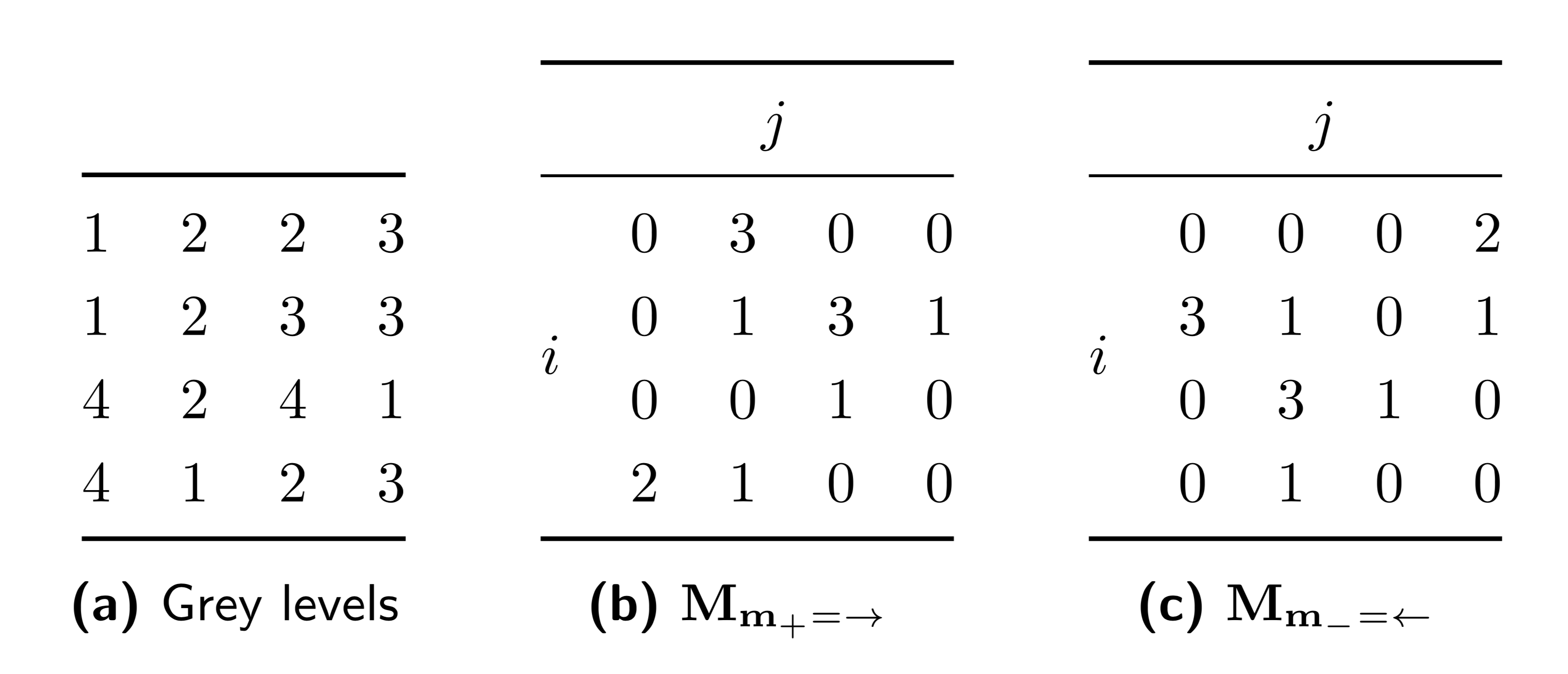
Fig. 10 Grey levels (a) and corresponding grey level co-occurrence matrices for the 0◦ (b) and 180◦ directions (c). In vector notation these directions are \(\mathbf{m_{+}} = (1, 0)\) and \(\mathbf{m_{-}}\) = (−1, 0). To calculate the symmetrical co-occurrence matrix \(\mathbf{M}_{\mathbf{m}}\) both matrices are summed by element.

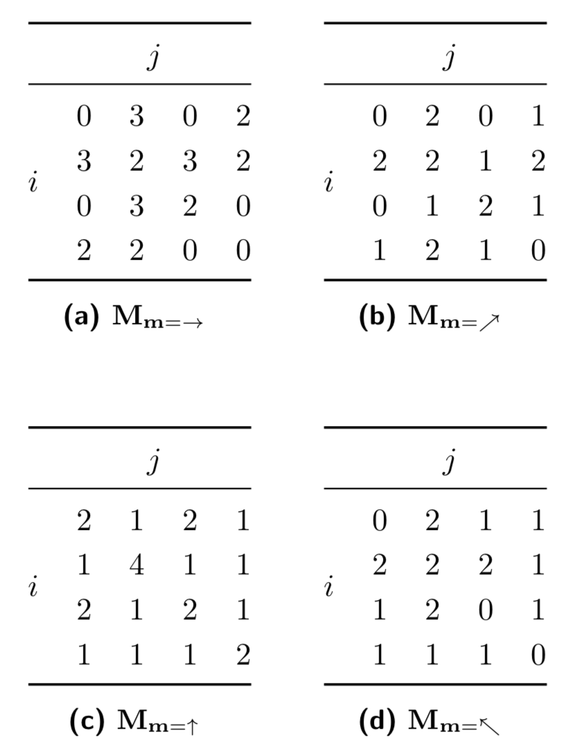
Fig. 11 Grey level co-occurrence matrices for the 0◦ (a), 45◦ (b), 90◦ (c) and 135◦ (d) directions. In vector notation these directions are \(\mathbf{m} = (1, 0)\), \(\mathbf{m} = (1, 1)\), \(\mathbf{m} = (0, 1)\) and \(\mathbf{m} = (−1, 1)\), respectively.

GLCM features rely on the probability distribution for the elements of the GLCM. Let us consider \(\mathbf{M}_{\mathbf{m}=(1,0)}\) from the example, as shown in Fig. 12. We derive a probability distribution for grey level co-occurrences, \(\mathbf{P}_{\mathbf{m}}\), by normalising \(\mathbf{M}_{\mathbf{m}}\) by the sum of its elements. Each element \(p_{ij}\) of \(\mathbf{P}_{\mathbf{m}}\) is then the joint probability of grey levels \(i\) and \(j\) occurring in neighbouring voxels along direction \(\mathbf{m}\). Then \(p_{i.} = \sum_{j=1}^{N_g} p_{ij}\) is the row marginal probability, and \(p_{.j}=\sum_{i=1}^{N_g} p_{ij}\) is the column marginal probability. As \(\mathbf{P}_{\mathbf{m}}\) is by definition symmetric, \(p_{i.} = p_{.j}\). Furthermore, let us consider diagonal and cross-diagonal probabilities \(p_{i-j}\) and \(p_{i+j}\) [Haralick1973][Unser1986]:

\[\begin{split}\begin{aligned} p_{i-j,k}&=\sum_{i=1}^{N_g} \sum_{j=1}^{N_g} p_{ij}\, \left[k=|i-j|\right]\qquad k=0,\ldots ,N_g-1\\ p_{i+j,k}&=\sum_{i=1}^{N_g} \sum_{j=1}^{N_g} p_{ij}\, \left[k=i+j\right]\qquad k=2,\ldots ,2N_g\end{aligned}\end{split}\]

Here, \(\left[\ldots\right]\) is an Iverson bracket, which equals \(1\) when the condition within the brackets is true and \(0\) otherwise. In effect we select only combinations of elements \((i,j)\) for which the condition holds.

It should be noted that while a distance \(\delta=1\) is commonly used for GLCM, other distances are possible. However, this does not change the number of For example, for \(\delta=3\) (in 3D) the voxels at \((0,0,3)\), \((0,3,0)\), \((3,0,0)\), \((0,3,3)\), \((0,3,-3)\), \((3,0,3)\), \((3,0,-3)\), \((3,3,0)\), \((3,-3,0)\), \((3,3,3)\), \((3,3,-3)\), \((3,-3,3)\) and \((3,-3,-3)\) from the center voxel are considered.

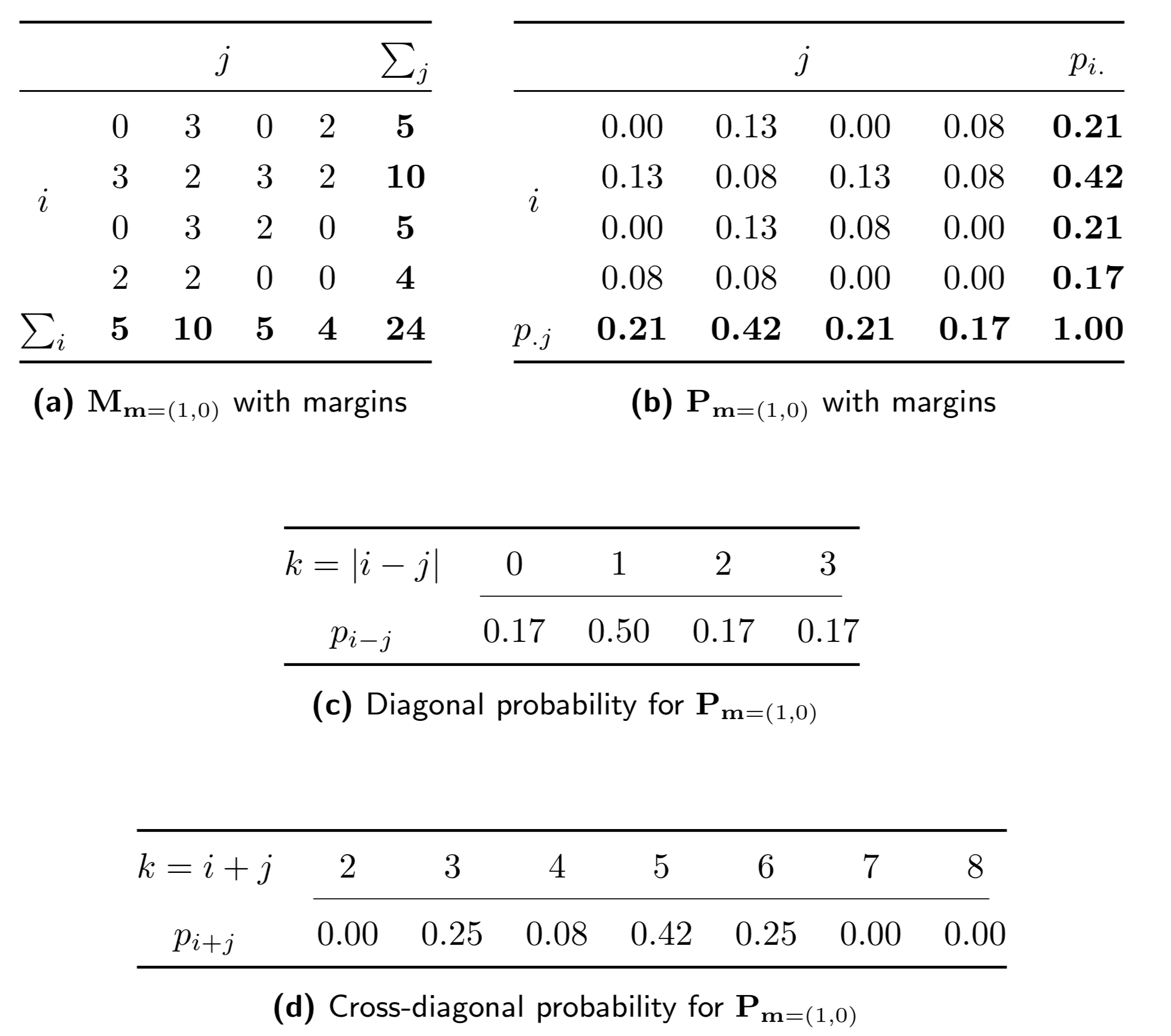
Fig. 12 Grey level co-occurrence matrix for the 0◦ direction (a); its corresponding probability matrix \(\mathbf{P}_{\mathbf{m}} = (1,0)\) with marginal probabilities \(p_{i.}\). and \(p_{.j}\); the diagonal probabilities \(p_{i-j}\) (c); and the cross-diagonal probabilities \(p_{i+j}\) (d). Discrepancies in panels b, c, and d are due to rounding errors caused by showing only two decimal places. Also, note that due to GLCM symmetry marginal probabilities \(p_{i.}\). and \(p_{.j}\) are the same in both row and column margins of panel b.

Aggregating features

To improve rotational invariance, GLCM feature values are computed by aggregating information from the different underlying directional matrices [Depeursinge2017a]. Five methods can be used to aggregate GLCMs and arrive at a single feature value. A schematic example is shown in Fig. 13. A feature may be aggregated as follows:

1. Features are computed from each 2D directional matrix and averaged over 2D directions and slices (BTW3).
2. Features are computed from a single matrix after merging 2D directional matrices per slice, and then averaged over slices (SUJT).
3. Features are computed from a single matrix after merging 2D directional matrices per direction, and then averaged over directions (JJUI).
4. The feature is computed from a single matrix after merging all 2D directional matrices (ZW7Z).
5. Features are computed from each 3D directional matrix and averaged over the 3D directions (ITBB).
6. The feature is computed from a single matrix after merging all 3D directional matrices (IAZD).

In methods 2,3,4 and 6, matrices are merged by summing the co-occurrence counts in each matrix element \((i,j)\) over the different matrices. Probability distributions are subsequently calculated for the merged GLCM, which is then used to calculate GLCM features. Feature values may dependent strongly on the aggregation method.

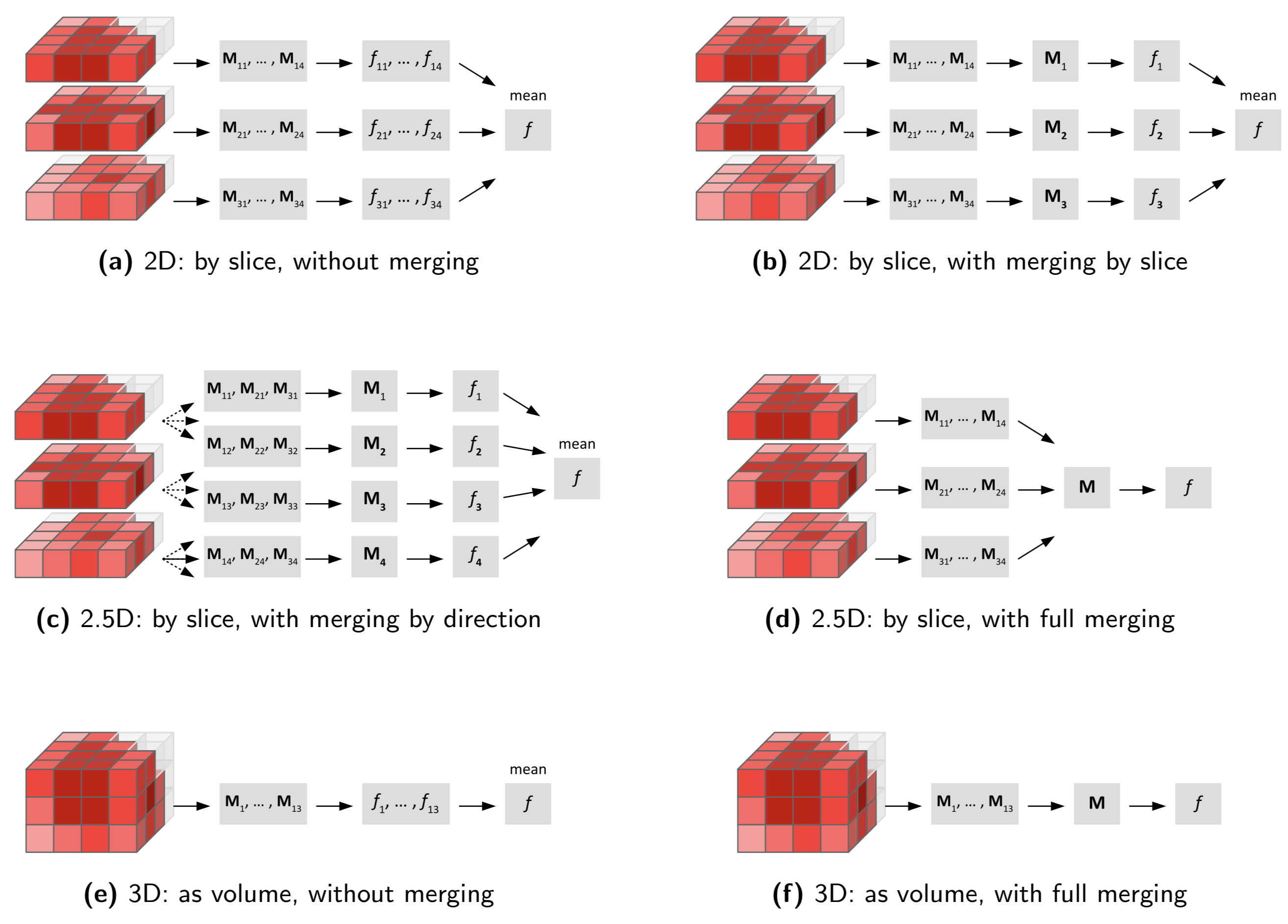
Fig. 13 Approaches to calculating grey level co-occurrence matrix-based features. M∆k are texture matrices calculated for direction \(\delta\) in slice \(k\) (if applicable), and \(f_{\delta k}\) is the corresponding feature value. In (b-d) and (e) the matrices are merged prior to feature calculation.

Distances and distance weighting

The default neighbourhood includes all voxels within Chebyshev distance \(1\). The corresponding direction vectors are multiplied by the desired distance \(\delta\). From a technical point-of-view, direction vectors may also be determined differently, using any distance norm. In this case, direction vectors are the vectors to the voxels at \(\delta\), or between \(\delta\) and \(\delta-1\) for the Euclidean norm. Such usage is however rare and we caution against it due to potential reproducibility issues.

GLCMs may be weighted for distance by multiplying \(\mathbf{M}\) with a weighting factor \(w\). By default \(w=1\), but \(w\) may also be an inverse distance function to weight each GLCM, e.g. \(w=\|\mathbf{m}\|^{-1}\) or \(w=\exp(-\|\mathbf{m}\|^2)\) [VanGriethuysen2017], with \(\|\mathbf{m}\|\) the length of direction vector \(m\). Whether distance weighting yields different feature values depends on several factors. When aggregating the feature values, matrices have to be merged first, otherwise weighting has no effect. Also, it has no effect if the default neighbourhood is used and the Chebyshev norm is using for weighting. Nor does weighting have an effect if either Manhattan or Chebyshev norms are used both for constructing a non-default neighbourhood and for weighting. Weighting may furthermore have no effect for distance \(\delta=1\), dependent on distance norms. Because of these exceptions, we recommend against using distance weighting for GLCM.

Joint maximum

GYBY

Joint maximum [Haralick1979] is the probability corresponding to the most common grey level co-occurrence in the GLCM:

\[F_{\mathit{cm.joint.max}}=\text{max}(p_{ij})\]

data	aggr. method	value	tol.	consensus
dig. phantom	2D, averaged	0.519	—	very strong
dig. phantom	2D, slice-merged	0.512	—	strong
dig. phantom	2.5D, direction-merged	0.489	—	strong
dig. phantom	2.5D, merged	0.492	—	strong
dig. phantom	3D, averaged	0.503	—	very strong
dig. phantom	3D, merged	0.509	—	very strong
config. A	2D, averaged	0.109	0.001	strong
config. A	2D, slice-merged	0.109	0.001	strong
config. A	2.5D, direction-merged	0.0943	0.0008	strong
config. A	2.5D, merged	0.0943	0.0008	strong
config. B	2D, averaged	0.156	0.002	strong
config. B	2D, slice-merged	0.156	0.002	strong
config. B	2.5D, direction-merged	0.126	0.002	strong
config. B	2.5D, merged	0.126	0.002	strong
config. C	3D, averaged	0.111	0.002	strong
config. C	3D, merged	0.111	0.002	very strong
config. D	3D, averaged	0.232	0.007	strong
config. D	3D, merged	0.232	0.007	strong
config. E	3D, averaged	0.153	0.003	moderate
config. E	3D, merged	0.153	0.003	strong

Joint average

60VM

Joint average [Unser1986] is the grey level weighted sum of joint probabilities:

\[F_{\mathit{cm.joint.avg}}=\sum_{i=1}^{N_g} \sum_{j=1}^{N_g} i\, p_{ij}\]

data	aggr. method	value	tol.	consensus
dig. phantom	2D, averaged	2.14	—	very strong
dig. phantom	2D, slice-merged	2.14	—	strong
dig. phantom	2.5D, direction-merged	2.2	—	strong
dig. phantom	2.5D, merged	2.2	—	strong
dig. phantom	3D, averaged	2.14	—	very strong
dig. phantom	3D, merged	2.15	—	very strong
config. A	2D, averaged	20.6	0.1	strong
config. A	2D, slice-merged	20.6	0.1	strong
config. A	2.5D, direction-merged	21.3	0.1	strong
config. A	2.5D, merged	21.3	0.1	strong
config. B	2D, averaged	18.7	0.3	strong
config. B	2D, slice-merged	18.7	0.3	strong
config. B	2.5D, direction-merged	19.2	0.3	strong
config. B	2.5D, merged	19.2	0.3	strong
config. C	3D, averaged	39	0.2	strong
config. C	3D, merged	39	0.2	strong
config. D	3D, averaged	18.9	0.5	strong
config. D	3D, merged	18.9	0.5	strong
config. E	3D, averaged	22.1	0.3	strong
config. E	3D, merged	22.1	0.3	strong

Joint variance

UR99

The joint variance [Unser1986], which is also called sum of squares [Haralick1973], is defined as:

\[F_{\mathit{cm.joint.var}}=\sum_{i=1}^{N_g} \sum_{j=1}^{N_g} \left(i-\mu\right)^2 p_{ij}\]

Here \(\mu\) is equal to the value of \(F_{\mathit{cm.joint.avg}}\), which was defined above.

data	aggr. method	value	tol.	consensus
dig. phantom	2D, averaged	2.69	—	very strong
dig. phantom	2D, slice-merged	2.71	—	strong
dig. phantom	2.5D, direction-merged	3.22	—	strong
dig. phantom	2.5D, merged	3.24	—	strong
dig. phantom	3D, averaged	3.1	—	very strong
dig. phantom	3D, merged	3.13	—	very strong
config. A	2D, averaged	27	0.4	strong
config. A	2D, slice-merged	27	0.4	strong
config. A	2.5D, direction-merged	18.6	0.5	strong
config. A	2.5D, merged	18.6	0.5	strong
config. B	2D, averaged	21	0.3	strong
config. B	2D, slice-merged	21	0.3	strong
config. B	2.5D, direction-merged	14.2	0.1	strong
config. B	2.5D, merged	14.2	0.1	strong
config. C	3D, averaged	73.7	2	strong
config. C	3D, merged	73.8	2	very strong
config. D	3D, averaged	17.6	0.4	strong
config. D	3D, merged	17.6	0.4	strong
config. E	3D, averaged	24.4	0.9	moderate
config. E	3D, merged	24.4	0.9	strong

Joint entropy

TU9B

Joint entropy [Haralick1973] is defined as:

\[F_{\mathit{cm.joint.entr}}=-\sum_{i=1}^{N_g} \sum_{j=1}^{N_g} p_{ij} \log_2 p_{ij}\]

data	aggr. method	value	tol.	consensus
dig. phantom	2D, averaged	2.05	—	very strong
dig. phantom	2D, slice-merged	2.24	—	strong
dig. phantom	2.5D, direction-merged	2.48	—	strong
dig. phantom	2.5D, merged	2.61	—	strong
dig. phantom	3D, averaged	2.4	—	very strong
dig. phantom	3D, merged	2.57	—	very strong
config. A	2D, averaged	5.82	0.04	strong
config. A	2D, slice-merged	5.9	0.04	strong
config. A	2.5D, direction-merged	5.78	0.04	strong
config. A	2.5D, merged	5.79	0.04	strong
config. B	2D, averaged	5.26	0.02	strong
config. B	2D, slice-merged	5.45	0.01	strong
config. B	2.5D, direction-merged	5.45	0.01	strong
config. B	2.5D, merged	5.46	0.01	strong
config. C	3D, averaged	6.39	0.06	strong
config. C	3D, merged	6.42	0.06	very strong
config. D	3D, averaged	4.95	0.03	strong
config. D	3D, merged	4.96	0.03	strong
config. E	3D, averaged	5.6	0.03	strong
config. E	3D, merged	5.61	0.03	strong

Difference average

TF7R

The difference average [Unser1986] for the diagonal probabilities is defined as:

\[F_{\mathit{cm.diff.avg}}=\sum_{k=0}^{N_g-1} k\, p_{i-j,k}\]

By definition difference average is equivalent to the dissimilarity feature [VanGriethuysen2017].

data	aggr. method	value	tol.	consensus
dig. phantom	2D, averaged	1.42	—	very strong
dig. phantom	2D, slice-merged	1.4	—	strong
dig. phantom	2.5D, direction-merged	1.46	—	strong
dig. phantom	2.5D, merged	1.44	—	strong
dig. phantom	3D, averaged	1.43	—	very strong
dig. phantom	3D, merged	1.38	—	very strong
config. A	2D, averaged	1.58	0.03	strong
config. A	2D, slice-merged	1.57	0.03	strong
config. A	2.5D, direction-merged	1.35	0.03	strong
config. A	2.5D, merged	1.35	0.03	strong
config. B	2D, averaged	1.81	0.01	strong
config. B	2D, slice-merged	1.81	0.01	strong
config. B	2.5D, direction-merged	1.47	0.01	strong
config. B	2.5D, merged	1.47	0.01	strong
config. C	3D, averaged	2.17	0.05	strong
config. C	3D, merged	2.16	0.05	strong
config. D	3D, averaged	1.29	0.01	strong
config. D	3D, merged	1.29	0.01	strong
config. E	3D, averaged	1.7	0.01	strong
config. E	3D, merged	1.7	0.01	strong

Difference variance

D3YU

The difference variance for the diagonal probabilities [Haralick1973] is defined as:

\[F_{\mathit{cm.diff.var}}=\sum_{k=0}^{N_g-1} (k-\mu)^2 p_{i-j,k}\]

Here \(\mu\) is equal to the value of difference average.

data	aggr. method	value	tol.	consensus
dig. phantom	2D, averaged	2.9	—	very strong
dig. phantom	2D, slice-merged	3.06	—	strong
dig. phantom	2.5D, direction-merged	3.11	—	strong
dig. phantom	2.5D, merged	3.23	—	strong
dig. phantom	3D, averaged	3.06	—	very strong
dig. phantom	3D, merged	3.21	—	very strong
config. A	2D, averaged	4.94	0.19	strong
config. A	2D, slice-merged	4.96	0.19	strong
config. A	2.5D, direction-merged	4.12	0.2	strong
config. A	2.5D, merged	4.14	0.2	strong
config. B	2D, averaged	7.74	0.05	strong
config. B	2D, slice-merged	7.76	0.05	strong
config. B	2.5D, direction-merged	6.48	0.06	strong
config. B	2.5D, merged	6.48	0.06	strong
config. C	3D, averaged	14.4	0.5	strong
config. C	3D, merged	14.4	0.5	strong
config. D	3D, averaged	5.37	0.11	strong
config. D	3D, merged	5.38	0.11	strong
config. E	3D, averaged	8.22	0.06	strong
config. E	3D, merged	8.23	0.06	strong

Difference entropy

NTRS

The difference entropy for the diagonal probabilities [Haralick1973] is defined as:

\[F_{\mathit{cm.diff.entr}}=-\sum_{k=0}^{N_g-1} p_{i-j,k} \log_2 p_{i-j,k}\]

data	aggr. method	value	tol.	consensus
dig. phantom	2D, averaged	1.4	—	very strong
dig. phantom	2D, slice-merged	1.49	—	strong
dig. phantom	2.5D, direction-merged	1.61	—	strong
dig. phantom	2.5D, merged	1.67	—	strong
dig. phantom	3D, averaged	1.56	—	very strong
dig. phantom	3D, merged	1.64	—	very strong
config. A	2D, averaged	2.27	0.03	strong
config. A	2D, slice-merged	2.28	0.03	strong
config. A	2.5D, direction-merged	2.16	0.03	strong
config. A	2.5D, merged	2.16	0.03	strong
config. B	2D, averaged	2.35	0.01	strong
config. B	2D, slice-merged	2.38	0.01	strong
config. B	2.5D, direction-merged	2.24	0.01	moderate
config. B	2.5D, merged	2.24	0.01	strong
config. C	3D, averaged	2.64	0.03	strong
config. C	3D, merged	2.64	0.03	very strong
config. D	3D, averaged	2.13	0.01	strong
config. D	3D, merged	2.14	0.01	strong
config. E	3D, averaged	2.39	0.01	strong
config. E	3D, merged	2.4	0.01	strong

Sum average

ZGXS

The sum average for the cross-diagonal probabilities [Haralick1973] is defined as:

\[F_{\mathit{cm.sum.avg}}=\sum_{k=2}^{2N_g} k\, p_{i+j,k}\]

By definition, \(F_{\mathit{cm.sum.avg}} = 2 F_{\mathit{cm.joint.avg}}\) [VanGriethuysen2017].

data	aggr. method	value	tol.	consensus
dig. phantom	2D, averaged	4.28	—	very strong
dig. phantom	2D, slice-merged	4.29	—	strong
dig. phantom	2.5D, direction-merged	4.41	—	strong
dig. phantom	2.5D, merged	4.41	—	strong
dig. phantom	3D, averaged	4.29	—	very strong
dig. phantom	3D, merged	4.3	—	very strong
config. A	2D, averaged	41.3	0.1	strong
config. A	2D, slice-merged	41.3	0.1	strong
config. A	2.5D, direction-merged	42.7	0.1	strong
config. A	2.5D, merged	42.7	0.1	strong
config. B	2D, averaged	37.4	0.5	strong
config. B	2D, slice-merged	37.4	0.5	strong
config. B	2.5D, direction-merged	38.5	0.6	strong
config. B	2.5D, merged	38.5	0.6	strong
config. C	3D, averaged	78	0.3	strong
config. C	3D, merged	78	0.3	strong
config. D	3D, averaged	37.7	0.8	strong
config. D	3D, merged	37.7	0.8	strong
config. E	3D, averaged	44.3	0.4	strong
config. E	3D, merged	44.3	0.4	strong

Sum variance

OEEB

The sum variance for the cross-diagonal probabilities [Haralick1973] is defined as:

\[F_{\mathit{cm.sum.var}}=\sum_{k=2}^{2N_g} (k-\mu)^2 p_{i+j,k}\]

Here \(\mu\) is equal to the value of sum average. Sum variance is mathematically identical to the cluster tendency feature [VanGriethuysen2017].

data	aggr. method	value	tol.	consensus
dig. phantom	2D, averaged	5.47	—	very strong
dig. phantom	2D, slice-merged	5.66	—	strong
dig. phantom	2.5D, direction-merged	7.48	—	strong
dig. phantom	2.5D, merged	7.65	—	strong
dig. phantom	3D, averaged	7.07	—	very strong
dig. phantom	3D, merged	7.41	—	very strong
config. A	2D, averaged	100	1	strong
config. A	2D, slice-merged	100	1	strong
config. A	2.5D, direction-merged	68.5	1.3	strong
config. A	2.5D, merged	68.5	1.3	strong
config. B	2D, averaged	72.1	1	strong
config. B	2D, slice-merged	72.3	1	strong
config. B	2.5D, direction-merged	48.1	0.4	strong
config. B	2.5D, merged	48.1	0.4	strong
config. C	3D, averaged	276	8	strong
config. C	3D, merged	276	8	very strong
config. D	3D, averaged	63.4	1.3	strong
config. D	3D, merged	63.5	1.3	strong
config. E	3D, averaged	86.6	3.3	moderate
config. E	3D, merged	86.7	3.3	strong

Sum entropy

P6QZ

The sum entropy for the cross-diagonal probabilities [Haralick1973] is defined as:

\[F_{\mathit{cm.sum.entr}}=-\sum_{k=2}^{2N_g} p_{i+j,k} \log_2 p_{i+j,k}\]

data	aggr. method	value	tol.	consensus
dig. phantom	2D, averaged	1.6	—	very strong
dig. phantom	2D, slice-merged	1.79	—	strong
dig. phantom	2.5D, direction-merged	2.01	—	strong
dig. phantom	2.5D, merged	2.14	—	strong
dig. phantom	3D, averaged	1.92	—	very strong
dig. phantom	3D, merged	2.11	—	very strong
config. A	2D, averaged	4.19	0.03	strong
config. A	2D, slice-merged	4.21	0.03	strong
config. A	2.5D, direction-merged	4.17	0.03	strong
config. A	2.5D, merged	4.18	0.03	strong
config. B	2D, averaged	3.83	0.01	strong
config. B	2D, slice-merged	3.89	0.01	strong
config. B	2.5D, direction-merged	3.91	0.01	strong
config. B	2.5D, merged	3.91	0.01	strong
config. C	3D, averaged	4.56	0.04	strong
config. C	3D, merged	4.56	0.04	very strong
config. D	3D, averaged	3.68	0.02	strong
config. D	3D, merged	3.68	0.02	strong
config. E	3D, averaged	3.96	0.02	strong
config. E	3D, merged	3.97	0.02	strong

Angular second moment

8ZQL

The angular second moment [Haralick1973], which represents the energy of \(\mathbf{P}_{\Delta}\), is defined as:

\[F_{\mathit{cm.energy}} = \sum_{i=1}^{N_g} \sum_{j=1}^{N_g} p_{ij}^2\]

This feature is also called energy [Unser1986][Aerts2014] and uniformity [Clausi2002].

data	aggr. method	value	tol.	consensus
dig. phantom	2D, averaged	0.368	—	very strong
dig. phantom	2D, slice-merged	0.352	—	strong
dig. phantom	2.5D, direction-merged	0.286	—	strong
dig. phantom	2.5D, merged	0.277	—	strong
dig. phantom	3D, averaged	0.303	—	very strong
dig. phantom	3D, merged	0.291	—	very strong
config. A	2D, averaged	0.045	0.0008	strong
config. A	2D, slice-merged	0.0446	0.0008	strong
config. A	2.5D, direction-merged	0.0429	0.0007	strong
config. A	2.5D, merged	0.0427	0.0007	strong
config. B	2D, averaged	0.0678	0.0006	strong
config. B	2D, slice-merged	0.0669	0.0006	strong
config. B	2.5D, direction-merged	0.0581	0.0006	strong
config. B	2.5D, merged	0.058	0.0006	strong
config. C	3D, averaged	0.045	0.001	strong
config. C	3D, merged	0.0447	0.001	very strong
config. D	3D, averaged	0.11	0.003	strong
config. D	3D, merged	0.109	0.003	strong
config. E	3D, averaged	0.0638	0.0009	strong
config. E	3D, merged	0.0635	0.0009	strong

Contrast

ACUI

Contrast assesses grey level variations [Haralick1973]. Hence elements of \(\mathbf{M}_{\Delta}\) that represent large grey level differences receive greater weight. Contrast is defined as [Clausi2002]:

\[F_{\mathit{cm.contrast}}= \sum_{i=1}^{N_g} \sum_{j=1}^{N_g} \left(i-j\right)^2 p_{ij}\]

Note that the original definition by [Haralick1973] is seemingly more complex, but rearranging and simplifying terms leads to the above formulation of contrast.

data	aggr. method	value	tol.	consensus
dig. phantom	2D, averaged	5.28	—	very strong
dig. phantom	2D, slice-merged	5.19	—	strong
dig. phantom	2.5D, direction-merged	5.39	—	strong
dig. phantom	2.5D, merged	5.29	—	strong
dig. phantom	3D, averaged	5.32	—	very strong
dig. phantom	3D, merged	5.12	—	very strong
config. A	2D, averaged	7.85	0.26	strong
config. A	2D, slice-merged	7.82	0.26	strong
config. A	2.5D, direction-merged	5.96	0.27	strong
config. A	2.5D, merged	5.95	0.27	strong
config. B	2D, averaged	11.9	0.1	strong
config. B	2D, slice-merged	11.8	0.1	strong
config. B	2.5D, direction-merged	8.66	0.09	strong
config. B	2.5D, merged	8.65	0.09	strong
config. C	3D, averaged	19.2	0.7	strong
config. C	3D, merged	19.1	0.7	very strong
config. D	3D, averaged	7.07	0.13	strong
config. D	3D, merged	7.05	0.13	strong
config. E	3D, averaged	11.1	0.1	strong
config. E	3D, merged	11.1	0.1	strong

Dissimilarity

8S9J

Dissimilarity [Clausi2002] is conceptually similar to the contrast feature, and is defined as:

\[F_{\mathit{cm.dissimilarity}}= \sum_{i=1}^{N_g} \sum_{j=1}^{N_g} |i-j|\, p_{ij}\]

By definition dissimilarity is equivalent to the difference average feature [VanGriethuysen2017].

data	aggr. method	value	tol.	consensus
dig. phantom	2D, averaged	1.42	—	very strong
dig. phantom	2D, slice-merged	1.4	—	strong
dig. phantom	2.5D, direction-merged	1.46	—	strong
dig. phantom	2.5D, merged	1.44	—	strong
dig. phantom	3D, averaged	1.43	—	very strong
dig. phantom	3D, merged	1.38	—	very strong
config. A	2D, averaged	1.58	0.03	strong
config. A	2D, slice-merged	1.57	0.03	strong
config. A	2.5D, direction-merged	1.35	0.03	strong
config. A	2.5D, merged	1.35	0.03	strong
config. B	2D, averaged	1.81	0.01	strong
config. B	2D, slice-merged	1.81	0.01	strong
config. B	2.5D, direction-merged	1.47	0.01	strong
config. B	2.5D, merged	1.47	0.01	strong
config. C	3D, averaged	2.17	0.05	strong
config. C	3D, merged	2.16	0.05	very strong
config. D	3D, averaged	1.29	0.01	strong
config. D	3D, merged	1.29	0.01	strong
config. E	3D, averaged	1.7	0.01	strong
config. E	3D, merged	1.7	0.01	strong

Inverse difference

IB1Z

Inverse difference is a measure of homogeneity [Clausi2002]. Grey level co-occurrences with a large difference in levels are weighed less, thus lowering the total feature value. The feature score is maximal if all grey levels are the same. Inverse difference is defined as:

\[F_{\mathit{cm.inv.diff}}=\sum_{i=1}^{N_g} \sum_{j=1}^{N_g} \frac{p_{ij}}{1+|i-j|}\]

The equation above may also be expressed in terms of diagonal probabilities [VanGriethuysen2017]:

\[F_{\mathit{cm.inv.diff}}=\sum_{k=0}^{N_g-1} \frac{p_{i-j,k}}{1+k}\]

data	aggr. method	value	tol.	consensus
dig. phantom	2D, averaged	0.678	—	very strong
dig. phantom	2D, slice-merged	0.683	—	strong
dig. phantom	2.5D, direction-merged	0.668	—	strong
dig. phantom	2.5D, merged	0.673	—	strong
dig. phantom	3D, averaged	0.677	—	very strong
dig. phantom	3D, merged	0.688	—	very strong
config. A	2D, averaged	0.581	0.003	strong
config. A	2D, slice-merged	0.581	0.003	strong
config. A	2.5D, direction-merged	0.605	0.003	strong
config. A	2.5D, merged	0.605	0.003	strong
config. B	2D, averaged	0.592	0.001	strong
config. B	2D, slice-merged	0.593	0.001	strong
config. B	2.5D, direction-merged	0.628	0.001	strong
config. B	2.5D, merged	0.628	0.001	strong
config. C	3D, averaged	0.582	0.004	strong
config. C	3D, merged	0.583	0.004	very strong
config. D	3D, averaged	0.682	0.003	strong
config. D	3D, merged	0.682	0.003	strong
config. E	3D, averaged	0.608	0.001	moderate
config. E	3D, merged	0.608	0.001	strong

Normalised inverse difference

NDRX

[Clausi2002] suggested normalising inverse difference to improve classification ability. The normalised feature is then defined as:

\[F_{\mathit{cm.inv.diff.norm}}=\sum_{i=1}^{N_g} \sum_{j=1}^{N_g} \frac{p_{ij}}{1+|i-j|/N_g}\]

Note that in Clausi’s definition, \(|i-j|^2/N_g^2\) is used instead of \(|i-j|/N_g\), which is likely an oversight, as this exactly matches the definition of the normalised inverse difference moment feature.

The equation may also be expressed in terms of diagonal probabilities [VanGriethuysen2017]:

\[F_{\mathit{cm.inv.diff.norm}}=\sum_{k=0}^{N_g-1} \frac{p_{i-j,k}}{1+k/N_g}\]

data	aggr. method	value	tol.	consensus
dig. phantom	2D, averaged	0.851	—	very strong
dig. phantom	2D, slice-merged	0.854	—	strong
dig. phantom	2.5D, direction-merged	0.847	—	strong
dig. phantom	2.5D, merged	0.85	—	strong
dig. phantom	3D, averaged	0.851	—	very strong
dig. phantom	3D, merged	0.856	—	very strong
config. A	2D, averaged	0.961	0.001	strong
config. A	2D, slice-merged	0.961	0.001	strong
config. A	2.5D, direction-merged	0.966	0.001	strong
config. A	2.5D, merged	0.966	0.001	strong
config. B	2D, averaged	0.952	0.001	strong
config. B	2D, slice-merged	0.952	0.001	strong
config. B	2.5D, direction-merged	0.96	0.001	strong
config. B	2.5D, merged	0.96	0.001	strong
config. C	3D, averaged	0.966	0.001	strong
config. C	3D, merged	0.966	0.001	very strong
config. D	3D, averaged	0.965	0.001	strong
config. D	3D, merged	0.965	0.001	strong
config. E	3D, averaged	0.955	0.001	strong
config. E	3D, merged	0.955	0.001	strong

Inverse difference moment

WF0Z

Inverse difference moment [Haralick1973] is similar in concept to the inverse difference feature, but with lower weights for elements that are further from the diagonal:

\[F_{\mathit{cm.inv.diff.mom}}=\sum_{i=1}^{N_g} \sum_{j=1}^{N_g} \frac{p_{ij}}{1+\left(i-j\right)^2}\]

The equation above may also be expressed in terms of diagonal probabilities [VanGriethuysen2017]:

\[F_{\mathit{cm.inv.diff.mom}}=\sum_{k=0}^{N_g-1} \frac{p_{i-j,k}}{1+k^2}\]

This feature is also called homogeneity [Unser1986].

data	aggr. method	value	tol.	consensus
dig. phantom	2D, averaged	0.619	—	very strong
dig. phantom	2D, slice-merged	0.625	—	strong
dig. phantom	2.5D, direction-merged	0.606	—	strong
dig. phantom	2.5D, merged	0.613	—	strong
dig. phantom	3D, averaged	0.618	—	very strong
dig. phantom	3D, merged	0.631	—	very strong
config. A	2D, averaged	0.544	0.003	strong
config. A	2D, slice-merged	0.544	0.003	strong
config. A	2.5D, direction-merged	0.573	0.003	strong
config. A	2.5D, merged	0.573	0.003	strong
config. B	2D, averaged	0.557	0.001	strong
config. B	2D, slice-merged	0.558	0.001	strong
config. B	2.5D, direction-merged	0.6	0.001	strong
config. B	2.5D, merged	0.6	0.001	strong
config. C	3D, averaged	0.547	0.004	strong
config. C	3D, merged	0.548	0.004	very strong
config. D	3D, averaged	0.656	0.003	strong
config. D	3D, merged	0.657	0.003	strong
config. E	3D, averaged	0.576	0.001	strong
config. E	3D, merged	0.577	0.001	strong

Normalised inverse difference moment

1QCO

[Clausi2002] suggested normalising inverse difference moment to improve classification performance. This leads to the following definition:

\[F_{\mathit{cm.inv.diff.mom.norm}}=\sum_{i=1}^{N_g} \sum_{j=1}^{N_g} \frac{p_{ij}}{1+\left(i-j\right)^2/N_g^2}\]

The equation above may also be expressed in terms of diagonal probabilities [VanGriethuysen2017]:

\[F_{\mathit{cm.inv.diff.mom.norm}}=\sum_{k=0}^{N_g-1} \frac{p_{i-j,k}}{1+\left(k/N_g\right)^2}\]

data	aggr. method	value	tol.	consensus
dig. phantom	2D, averaged	0.899	—	very strong
dig. phantom	2D, slice-merged	0.901	—	strong
dig. phantom	2.5D, direction-merged	0.897	—	strong
dig. phantom	2.5D, merged	0.899	—	strong
dig. phantom	3D, averaged	0.898	—	very strong
dig. phantom	3D, merged	0.902	—	very strong
config. A	2D, averaged	0.994	0.001	strong
config. A	2D, slice-merged	0.994	0.001	strong
config. A	2.5D, direction-merged	0.996	0.001	strong
config. A	2.5D, merged	0.996	0.001	strong
config. B	2D, averaged	0.99	0.001	strong
config. B	2D, slice-merged	0.99	0.001	strong
config. B	2.5D, direction-merged	0.992	0.001	strong
config. B	2.5D, merged	0.992	0.001	strong
config. C	3D, averaged	0.994	0.001	strong
config. C	3D, merged	0.994	0.001	very strong
config. D	3D, averaged	0.994	0.001	strong
config. D	3D, merged	0.994	0.001	strong
config. E	3D, averaged	0.99	0.001	strong
config. E	3D, merged	0.99	0.001	strong

Inverse variance

E8JP

The inverse variance [Aerts2014] feature is defined as:

\[F_{\mathit{cm.inv.var}}=2\sum_{i=1}^{N_g} \sum_{j>i}^{N_g} \frac{p_{ij}}{\left(i-j\right)^2}\]

The equation above may also be expressed in terms of diagonal probabilities. Note that in this case, summation starts at \(k=1\) instead of \(k=0\)[VanGriethuysen2017]:

\[F_{\mathit{cm.inv.var}}=\sum_{k=1}^{N_g-1} \frac{p_{i-j,k}}{k^2}\]

data	aggr. method	value	tol.	consensus
dig. phantom	2D, averaged	0.0567	—	very strong
dig. phantom	2D, slice-merged	0.0553	—	strong
dig. phantom	2.5D, direction-merged	0.0597	—	strong
dig. phantom	2.5D, merged	0.0582	—	strong
dig. phantom	3D, averaged	0.0604	—	very strong
dig. phantom	3D, merged	0.0574	—	very strong
config. A	2D, averaged	0.441	0.001	strong
config. A	2D, slice-merged	0.441	0.001	strong
config. A	2.5D, direction-merged	0.461	0.002	strong
config. A	2.5D, merged	0.461	0.002	strong
config. B	2D, averaged	0.401	0.002	strong
config. B	2D, slice-merged	0.401	0.002	strong
config. B	2.5D, direction-merged	0.424	0.003	strong
config. B	2.5D, merged	0.424	0.003	strong
config. C	3D, averaged	0.39	0.003	strong
config. C	3D, merged	0.39	0.003	very strong
config. D	3D, averaged	0.341	0.005	strong
config. D	3D, merged	0.34	0.005	strong
config. E	3D, averaged	0.41	0.004	strong
config. E	3D, merged	0.41	0.004	strong

Correlation

NI2N

Correlation [Haralick1973] is defined as:

\[F_{\mathit{cm.corr}}=\frac{1}{\sigma_{i.}\,\sigma_{.j}} \left(-\mu_{i.}\,\mu_{.j} + \sum_{i=1}^{N_g} \sum_{j=1}^{N_g} i\,j\,p_{ij}\right)\]

\(\mu_{i.}=\sum_{i=1}^{N_g}i\,p_{i.}\) and \(\sigma_{i.}=\left(\sum_{i=1}^{N_g} (i-\mu_{i.})^2 p_{i.}\right)^{1/2}\) are the mean and standard deviation of row marginal probability \(p_{i.}\), respectively. Likewise, \(\mu_{.j}\) and \(\sigma_{.j}\) are the mean and standard deviation of the column marginal probability \(p_{.j}\), respectively. The calculation of correlation can be simplified since \(\mathbf{P}_{\Delta}\) is symmetrical:

\[F_{\mathit{cm.corr}}=\frac{1}{\sigma_{i.}^2} \left(-\mu_{i.}^2 + \sum_{i=1}^{N_g} \sum_{j=1}^{N_g} i\,j\,p_{ij}\right)\]

An equivalent formulation of correlation is:

\[F_{\mathit{cm.corr}}=\frac{1}{\sigma_{i.}\,\sigma_{.j}} \sum_{i=1}^{N_g} \sum_{j=1}^{N_g} \left(i-\mu_{i.}\right) \left(j-\mu_{.j}\right)p_{ij}\]

Again, simplifying due to matrix symmetry yields:

\[F_{\mathit{cm.corr}}=\frac{1}{\sigma_{i.}^2} \sum_{i=1}^{N_g} \sum_{j=1}^{N_g} \left(i-\mu_{i.}\right) \left(j-\mu_{i.}\right)p_{ij}\]

data	aggr. method	value	tol.	consensus
dig. phantom	2D, averaged	\(-\)0.0121	—	very strong
dig. phantom	2D, slice-merged	0.0173	—	strong
dig. phantom	2.5D, direction-merged	0.178	—	strong
dig. phantom	2.5D, merged	0.182	—	strong
dig. phantom	3D, averaged	0.157	—	very strong
dig. phantom	3D, merged	0.183	—	very strong
config. A	2D, averaged	0.778	0.002	strong
config. A	2D, slice-merged	0.78	0.002	strong
config. A	2.5D, direction-merged	0.839	0.003	strong
config. A	2.5D, merged	0.84	0.003	strong
config. B	2D, averaged	0.577	0.002	strong
config. B	2D, slice-merged	0.58	0.002	strong
config. B	2.5D, direction-merged	0.693	0.003	strong
config. B	2.5D, merged	0.695	0.003	strong
config. C	3D, averaged	0.869	0.001	strong
config. C	3D, merged	0.871	0.001	strong
config. D	3D, averaged	0.798	0.005	strong
config. D	3D, merged	0.8	0.005	strong
config. E	3D, averaged	0.771	0.006	moderate
config. E	3D, merged	0.773	0.006	strong

Autocorrelation

QWB0

[soh1999texture] defined autocorrelation as:

\[F_{\mathit{cm.auto.corr}}=\sum_{i=1}^{N_g} \sum_{j=1}^{N_g} i\,j\,p_{ij}\]

data	aggr. method	value	tol.	consensus
dig. phantom	2D, averaged	5.09	—	very strong
dig. phantom	2D, slice-merged	5.14	—	strong
dig. phantom	2.5D, direction-merged	5.4	—	strong
dig. phantom	2.5D, merged	5.45	—	strong
dig. phantom	3D, averaged	5.06	—	very strong
dig. phantom	3D, merged	5.19	—	very strong
config. A	2D, averaged	455	2	strong
config. A	2D, slice-merged	455	2	strong
config. A	2.5D, direction-merged	471	2	strong
config. A	2.5D, merged	471	2	strong
config. B	2D, averaged	369	11	strong
config. B	2D, slice-merged	369	11	strong
config. B	2.5D, direction-merged	380	11	strong
config. B	2.5D, merged	380	11	strong
config. C	3D, averaged	\(1.58 \times 10^{3}\)	10	strong
config. C	3D, merged	\(1.58 \times 10^{3}\)	10	strong
config. D	3D, averaged	370	16	strong
config. D	3D, merged	370	16	very strong
config. E	3D, averaged	509	8	strong
config. E	3D, merged	509	8	strong

Cluster tendency

DG8W

Cluster tendency [Aerts2014] is defined as:

\[F_{\mathit{cm.clust.tend}}=\sum_{i=1}^{N_g} \sum_{j=1}^{N_g} \left(i+j-\mu_{i.}-\mu_{.j}\right)^2 p_{ij}\]

Here \(\mu_{i.}=\sum_{i=1}^{N_g} i\, p_{i.}\) and \(\mu_{.j}=\sum_{j=1}^{N_g} j\, p_{.j}\). Because of the symmetric nature of \(\mathbf{P}_{\Delta}\), the feature can also be formulated as:

\[F_{\mathit{cm.clust.tend}}=\sum_{i=1}^{N_g} \sum_{j=1}^{N_g} \left(i+j-2\mu_{i.}\right)^2 p_{ij}\]

Cluster tendency is mathematically equal to the sum variance feature [VanGriethuysen2017].

data	aggr. method	value	tol.	consensus
dig. phantom	2D, averaged	5.47	—	very strong
dig. phantom	2D, slice-merged	5.66	—	strong
dig. phantom	2.5D, direction-merged	7.48	—	strong
dig. phantom	2.5D, merged	7.65	—	strong
dig. phantom	3D, averaged	7.07	—	very strong
dig. phantom	3D, merged	7.41	—	very strong
config. A	2D, averaged	100	1	strong
config. A	2D, slice-merged	100	1	strong
config. A	2.5D, direction-merged	68.5	1.3	strong
config. A	2.5D, merged	68.5	1.3	strong
config. B	2D, averaged	72.1	1	strong
config. B	2D, slice-merged	72.3	1	strong
config. B	2.5D, direction-merged	48.1	0.4	strong
config. B	2.5D, merged	48.1	0.4	strong
config. C	3D, averaged	276	8	strong
config. C	3D, merged	276	8	very strong
config. D	3D, averaged	63.4	1.3	strong
config. D	3D, merged	63.5	1.3	strong
config. E	3D, averaged	86.6	3.3	moderate
config. E	3D, merged	86.7	3.3	strong

Cluster shade

7NFM

Cluster shade [Unser1986] is defined as:

\[F_{\mathit{cm.clust.shade}}=\sum_{i=1}^{N_g} \sum_{j=1}^{N_g} \left(i+j-\mu_{i.}-\mu_{.j}\right)^3 p_{ij}\]

As with cluster tendency, \(\mu_{i.}=\sum_{i=1}^{N_g} i\, p_{i.}\) and \(\mu_{.j}=\sum_{j=1}^{N_g} j\, p_{.j}\). Because of the symmetric nature of \(\mathbf{P}_{\Delta}\), the feature can also be formulated as:

\[F_{\mathit{cm.clust.shade}}=\sum_{i=1}^{N_g} \sum_{j=1}^{N_g} \left(i+j-2\mu_{i.}\right)^3 p_{ij}\]

data	aggr. method	value	tol.	consensus
dig. phantom	2D, averaged	7	—	very strong
dig. phantom	2D, slice-merged	6.98	—	strong
dig. phantom	2.5D, direction-merged	16.6	—	strong
dig. phantom	2.5D, merged	16.4	—	strong
dig. phantom	3D, averaged	16.6	—	very strong
dig. phantom	3D, merged	17.4	—	very strong
config. A	2D, averaged	\(-1.04 \times 10^{3}\)	20	strong
config. A	2D, slice-merged	\(-1.05 \times 10^{3}\)	20	strong
config. A	2.5D, direction-merged	\(-1.49 \times 10^{3}\)	30	strong
config. A	2.5D, merged	\(-1.49 \times 10^{3}\)	30	strong
config. B	2D, averaged	\(-\)668	17	strong
config. B	2D, slice-merged	\(-\)673	17	strong
config. B	2.5D, direction-merged	\(-\)905	19	strong
config. B	2.5D, merged	\(-\)906	19	strong
config. C	3D, averaged	\(-1.06 \times 10^{4}\)	300	strong
config. C	3D, merged	\(-1.06 \times 10^{4}\)	300	very strong
config. D	3D, averaged	\(-1.27 \times 10^{3}\)	40	strong
config. D	3D, merged	\(-1.28 \times 10^{3}\)	40	strong
config. E	3D, averaged	\(-2.07 \times 10^{3}\)	70	moderate
config. E	3D, merged	\(-2.08 \times 10^{3}\)	70	strong

Cluster prominence

AE86

Cluster prominence [Unser1986] is defined as:

\[F_{\mathit{cm.clust.prom}}=\sum_{i=1}^{N_g} \sum_{j=1}^{N_g} \left(i+j-\mu_{i.}-\mu_{.j}\right)^4 p_{ij}\]

As before, \(\mu_{i.}=\sum_{i=1}^{N_g} i\, p_{i.}\) and \(\mu_{.j}=\sum_{j=1}^{N_g} j\, p_{.j}\). Because of the symmetric nature of \(\mathbf{P}_{\Delta}\), the feature can also be formulated as:

\[F_{\mathit{cm.clust.prom}}=\sum_{i=1}^{N_g} \sum_{j=1}^{N_g} \left(i+j-2\mu_{i.}\right)^4 p_{ij}\]

data	aggr. method	value	tol.	consensus
dig. phantom	2D, averaged	79.1	—	very strong
dig. phantom	2D, slice-merged	80.4	—	strong
dig. phantom	2.5D, direction-merged	147	—	strong
dig. phantom	2.5D, merged	142	—	strong
dig. phantom	3D, averaged	145	—	very strong
dig. phantom	3D, merged	147	—	very strong
config. A	2D, averaged	\(5.27 \times 10^{4}\)	500	strong
config. A	2D, slice-merged	\(5.28 \times 10^{4}\)	500	strong
config. A	2.5D, direction-merged	\(4.76 \times 10^{4}\)	700	strong
config. A	2.5D, merged	\(4.77 \times 10^{4}\)	700	strong
config. B	2D, averaged	\(2.94 \times 10^{4}\)	\(1.4 \times 10^{3}\)	strong
config. B	2D, slice-merged	\(2.95 \times 10^{4}\)	\(1.4 \times 10^{3}\)	strong
config. B	2.5D, direction-merged	\(2.52 \times 10^{4}\)	\(1 \times 10^{3}\)	strong
config. B	2.5D, merged	\(2.53 \times 10^{4}\)	\(1 \times 10^{3}\)	strong
config. C	3D, averaged	\(5.69 \times 10^{5}\)	\(1.1 \times 10^{4}\)	strong
config. C	3D, merged	\(5.7 \times 10^{5}\)	\(1.1 \times 10^{4}\)	very strong
config. D	3D, averaged	\(3.57 \times 10^{4}\)	\(1.4 \times 10^{3}\)	strong
config. D	3D, merged	\(3.57 \times 10^{4}\)	\(1.5 \times 10^{3}\)	very strong
config. E	3D, averaged	\(6.89 \times 10^{4}\)	\(2.1 \times 10^{3}\)	moderate
config. E	3D, merged	\(6.9 \times 10^{4}\)	\(2.1 \times 10^{3}\)	strong

Information correlation 1

R8DG

Information theoretic correlation is estimated using two different measures [Haralick1973]. For symmetric \(\mathbf{P}_{\Delta}\) the first measure is defined as:

\[F_{\mathit{cm.info.corr.1}}=\frac{\mathit{HXY}-\mathit{HXY_1}}{\mathit{HX}}\]

\(\mathit{HXY} = -\sum_{i=1}^{N_g} \sum_{j=1}^{N_g} p_{ij} \log_2 p_{ij}\) is the entropy for the joint probability. \(\mathit{HX}=-\sum_{i=1}^{N_g} p_{i.} \log_2 p_{i.}\) is the entropy for the row marginal probability, which due to symmetry is equal to the entropy of the column marginal probability. \(\mathit{HXY}_1\) is a type of entropy that is defined as:

\[\mathit{HXY}_1 = -\sum_{i=1}^{N_g} \sum_{j=1}^{N_g} p_{ij} \log_2 \left(p_{i.} p_{.j}\right)\]

data	aggr. method	value	tol.	consensus
dig. phantom	2D, averaged	\(-\)0.155	—	very strong
dig. phantom	2D, slice-merged	\(-\)0.0341	—	strong
dig. phantom	2.5D, direction-merged	\(-\)0.124	—	strong
dig. phantom	2.5D, merged	\(-\)0.0334	—	strong
dig. phantom	3D, averaged	\(-\)0.157	—	very strong
dig. phantom	3D, merged	\(-\)0.0288	—	very strong
config. A	2D, averaged	\(-\)0.236	0.001	strong
config. A	2D, slice-merged	\(-\)0.214	0.001	strong
config. A	2.5D, direction-merged	\(-\)0.231	0.001	strong
config. A	2.5D, merged	\(-\)0.228	0.001	strong
config. B	2D, averaged	\(-\)0.239	0.001	strong
config. B	2D, slice-merged	\(-\)0.181	0.001	strong
config. B	2.5D, direction-merged	\(-\)0.188	0.001	strong
config. B	2.5D, merged	\(-\)0.185	0.001	strong
config. C	3D, averaged	\(-\)0.236	0.001	strong
config. C	3D, merged	\(-\)0.228	0.001	very strong
config. D	3D, averaged	\(-\)0.231	0.003	strong
config. D	3D, merged	\(-\)0.225	0.003	strong
config. E	3D, averaged	\(-\)0.181	0.003	moderate
config. E	3D, merged	\(-\)0.175	0.003	strong

Information correlation 2

JN9H

The second measure of information theoretic correlation [Haralick1973] is estimated as follows for symmetric \(\mathbf{P}_{\Delta}\):

\[F_{\mathit{cm.info.corr.2}}=\sqrt{1-\exp\left(-2\left(\mathit{HXY}_2-\mathit{HXY}\right)\right)}\]

As earlier, \(\mathit{HXY} = -\sum_{i=1}^{N_g} \sum_{j=1}^{N_g} p_{ij} \log_2 p_{ij}\). \(\mathit{HXY}_2\) is a type of entropy defined as:

\[\mathit{HXY}_2=-\sum_{i=1}^{N_g} \sum_{j=1}^{N_g} p_{i.} p_{.j} \log_2 \left(p_{i.} p_{.j} \right)\]

data	aggr. method	value	tol.	consensus
dig. phantom	2D, averaged	0.487	—	strong
dig. phantom	2D, slice-merged	0.263	—	strong
dig. phantom	2.5D, direction-merged	0.487	—	strong
dig. phantom	2.5D, merged	0.291	—	strong
dig. phantom	3D, averaged	0.52	—	very strong
dig. phantom	3D, merged	0.269	—	very strong
config. A	2D, averaged	0.863	0.003	strong
config. A	2D, slice-merged	0.851	0.002	strong
config. A	2.5D, direction-merged	0.879	0.001	strong
config. A	2.5D, merged	0.88	0.001	strong
config. B	2D, averaged	0.837	0.001	strong
config. B	2D, slice-merged	0.792	0.001	strong
config. B	2.5D, direction-merged	0.821	0.001	strong
config. B	2.5D, merged	0.819	0.001	strong
config. C	3D, averaged	0.9	0.001	strong
config. C	3D, merged	0.899	0.001	very strong
config. D	3D, averaged	0.845	0.003	strong
config. D	3D, merged	0.846	0.003	very strong
config. E	3D, averaged	0.813	0.004	moderate
config. E	3D, merged	0.813	0.004	strong

Grey level run length based features

TP0I

The grey level run length matrix (GLRLM) was introduced by [Galloway1975] to define various texture features. Like the grey level co-occurrence matrix, GLRLM also assesses the distribution of discretised grey levels in an image or in a stack of images. However, whereas GLCM assesses co-occurrence of grey levels within neighbouring pixels or voxels, GLRLM assesses run lengths. A run length is defined as the length of a consecutive sequence of pixels or voxels with the same grey level along direction \(\mathbf{m}\), which was previously defined in Grey level co-occurrence based features. The GLRLM then contains the occurrences of runs with length \(j\) for a discretised grey level \(i\).

A complete example for GLRLM construction from a 2D image is shown in Fig. 14. Let \(\mathbf{M}_{\mathbf{m}}\) be the \(N_g \times N_r\) grey level run length matrix, where \(N_g\) is the number of discretised grey levels present in the ROI intensity mask and \(N_r\) the maximal possible run length along direction \(\mathbf{m}\). Matrix element \(r_{ij}\) of the GLRLM is the occurrence of grev level \(i\) with run length \(j\). Then, let \(N_v\) be the total number of voxels in the ROI intensity mask, and \(N_s=\sum_{i=1}^{N_g}\sum_{j=1}^{N_r}r_{ij}\) the sum over all elements in \(\mathbf{M}_{\mathbf{m}}\). Marginal sums are also defined. Let \(r_{i.}\) be the marginal sum of the runs over run lengths \(j\) for grey value \(i\), that is \(r_{i.}=\sum_{j=1}^{N_r} r_{ij}\). Similarly, the marginal sum of the runs over the grey values \(i\) for run length \(j\) is \(r_{.j}=\sum_{i=1}^{N_g} r_{ij}\).

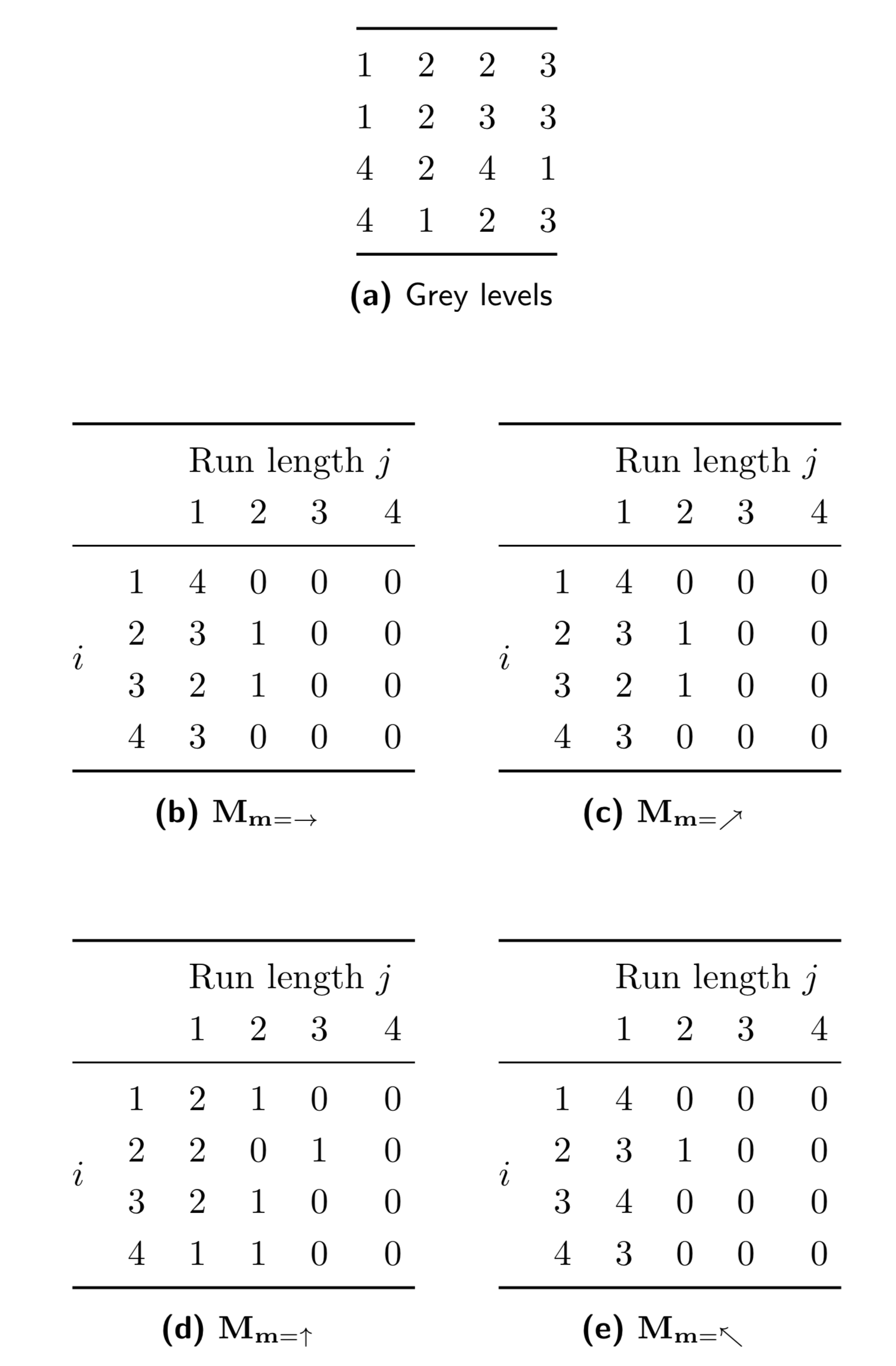
Fig. 14 Grey level run length matrices for the 0◦ (a), 45◦ (b), 90◦ (c) and 135◦ (d) directions. In vector notation these directions are \(\mathbf{m} = (1, 0)\), \(\mathbf{m} = (1, 1)\), \(\mathbf{m} = (0, 1)\) and \(\mathbf{m} = (-1, 1)\), respectively.

Aggregating features

To improve rotational invariance, GLRLM feature values are computed by aggregating information from the different underlying directional matrices [Depeursinge2017a]. Five methods can be used to aggregate GLRLMs and arrive at a single feature value. A schematic example was previously shown Fig. 13. A feature may be aggregated as follows:

1. Features are computed from each 2D directional matrix and averaged over 2D directions and slices (BTW3).
2. Features are computed from a single matrix after merging 2D directional matrices per slice, and then averaged over slices (SUJT).
3. Features are computed from a single matrix after merging 2D directional matrices per direction, and then averaged over directions (JJUI).
4. The feature is computed from a single matrix after merging all 2D directional matrices (ZW7Z).
5. Features are computed from each 3D directional matrix and averaged over the 3D directions (ITBB).
6. The feature is computed from a single matrix after merging all 3D directional matrices (IAZD).

In methods 2,3,4 and 6 matrices are merged by summing the run counts of each matrix element \((i,j)\) over the different matrices. Note that when matrices are merged, \(N_v\) should likewise be summed to retain consistency. Feature values may dependent strongly on the aggregation method.

Distance weighting

GLRLMs may be weighted for distance by multiplying the run lengths with a weighting factor \(w\). By default \(w=1\), but \(w\) may also be an inverse distance function, e.g. \(w=\|\mathbf{m}\|^{-1}\) or \(w=\exp(-\|\mathbf{m}\|^2)\) [VanGriethuysen2017], with \(\|\mathbf{m}\|\) the length of direction vector \(m\). Whether distance weighting yields different feature values depends on several factors. When aggregating the feature values, matrices have to be merged first, otherwise weighting has no effect. It also has no effect if the Chebyshev norm is used for weighting. Distance weighting is non-standard use, and we caution against it due to potential reproducibility issues.

Short runs emphasis

22OV

This feature emphasises short run lengths [Galloway1975]. It is defined as:

\[F_{\mathit{rlm.sre}} = \frac{1}{N_s} \sum_{j=1}^{N_r} \frac{r_{.j}}{j^2}\]

data	aggr. method	value	tol.	consensus
dig. phantom	2D, averaged	0.641	—	very strong
dig. phantom	2D, slice-merged	0.661	—	strong
dig. phantom	2.5D, direction-merged	0.665	—	strong
dig. phantom	2.5D, merged	0.68	—	strong
dig. phantom	3D, averaged	0.705	—	very strong
dig. phantom	3D, merged	0.729	—	very strong
config. A	2D, averaged	0.785	0.003	strong
config. A	2D, slice-merged	0.786	0.003	strong
config. A	2.5D, direction-merged	0.768	0.003	strong
config. A	2.5D, merged	0.769	0.003	strong
config. B	2D, averaged	0.781	0.001	strong
config. B	2D, slice-merged	0.782	0.001	strong
config. B	2.5D, direction-merged	0.759	0.001	strong
config. B	2.5D, merged	0.759	0.001	strong
config. C	3D, averaged	0.786	0.003	strong
config. C	3D, merged	0.787	0.003	strong
config. D	3D, averaged	0.734	0.001	strong
config. D	3D, merged	0.736	0.001	strong
config. E	3D, averaged	0.776	0.001	moderate
config. E	3D, merged	0.777	0.001	strong

Long runs emphasis

W4KF

This feature emphasises long run lengths [Galloway1975]. It is defined as:

\[F_{\mathit{rlm.lre}} = \frac{1}{N_s} \sum_{j=1}^{N_r} j^2 r_{.j}\]

data	aggr. method	value	tol.	consensus
dig. phantom	2D, averaged	3.78	—	very strong
dig. phantom	2D, slice-merged	3.51	—	strong
dig. phantom	2.5D, direction-merged	3.46	—	strong
dig. phantom	2.5D, merged	3.27	—	strong
dig. phantom	3D, averaged	3.06	—	very strong
dig. phantom	3D, merged	2.76	—	very strong
config. A	2D, averaged	2.91	0.03	strong
config. A	2D, slice-merged	2.89	0.03	strong
config. A	2.5D, direction-merged	3.09	0.03	strong
config. A	2.5D, merged	3.08	0.03	strong
config. B	2D, averaged	3.52	0.04	strong
config. B	2D, slice-merged	3.5	0.04	strong
config. B	2.5D, direction-merged	3.82	0.05	strong
config. B	2.5D, merged	3.81	0.05	strong
config. C	3D, averaged	3.31	0.04	strong
config. C	3D, merged	3.28	0.04	strong
config. D	3D, averaged	6.66	0.18	strong
config. D	3D, merged	6.56	0.18	strong
config. E	3D, averaged	3.55	0.07	strong
config. E	3D, merged	3.52	0.07	strong

Low grey level run emphasis

V3SW

This feature is a grey level analogue to short runs emphasis [Chu1990]. Instead of short run lengths, low grey levels are emphasised. The feature is defined as:

\[F_{\mathit{rlm.lgre}}=\frac{1}{N_s} \sum_{i=1}^{N_g} \frac{r_{i.}}{i^2}\]

data	aggr. method	value	tol.	consensus
dig. phantom	2D, averaged	0.604	—	very strong
dig. phantom	2D, slice-merged	0.609	—	strong
dig. phantom	2.5D, direction-merged	0.58	—	strong
dig. phantom	2.5D, merged	0.585	—	strong
dig. phantom	3D, averaged	0.603	—	very strong
dig. phantom	3D, merged	0.607	—	very strong
config. A	2D, averaged	0.0264	0.0003	strong
config. A	2D, slice-merged	0.0264	0.0003	strong
config. A	2.5D, direction-merged	0.0148	0.0004	strong
config. A	2.5D, merged	0.0147	0.0004	strong
config. B	2D, averaged	0.0331	0.0006	strong
config. B	2D, slice-merged	0.033	0.0006	strong
config. B	2.5D, direction-merged	0.0194	0.0006	strong
config. B	2.5D, merged	0.0194	0.0006	strong
config. C	3D, averaged	0.00155	\(5 \times 10^{-5}\)	strong
config. C	3D, merged	0.00155	\(5 \times 10^{-5}\)	strong
config. D	3D, averaged	0.0257	0.0012	strong
config. D	3D, merged	0.0257	0.0012	strong
config. E	3D, averaged	0.0204	0.0008	moderate
config. E	3D, merged	0.0204	0.0008	strong

High grey level run emphasis

G3QZ

The high grey level run emphasis feature is a grey level analogue to long runs emphasis [Chu1990]. The feature emphasises high grey levels, and is defined as:

\[F_{\mathit{rlm.hgre}}=\frac{1}{N_s} \sum_{i=1}^{N_g} i^2 r_{i.}\]

data	aggr. method	value	tol.	consensus
dig. phantom	2D, averaged	9.82	—	very strong
dig. phantom	2D, slice-merged	9.74	—	strong
dig. phantom	2.5D, direction-merged	10.3	—	strong
dig. phantom	2.5D, merged	10.2	—	strong
dig. phantom	3D, averaged	9.7	—	very strong
dig. phantom	3D, merged	9.64	—	very strong
config. A	2D, averaged	428	3	strong
config. A	2D, slice-merged	428	3	strong
config. A	2.5D, direction-merged	449	3	strong
config. A	2.5D, merged	449	3	strong
config. B	2D, averaged	342	11	strong
config. B	2D, slice-merged	342	11	strong
config. B	2.5D, direction-merged	356	11	strong
config. B	2.5D, merged	356	11	strong
config. C	3D, averaged	\(1.47 \times 10^{3}\)	10	strong
config. C	3D, merged	\(1.47 \times 10^{3}\)	10	strong
config. D	3D, averaged	326	17	strong
config. D	3D, merged	326	17	strong
config. E	3D, averaged	471	9	strong
config. E	3D, merged	471	9	strong

Short run low grey level emphasis

HTZT

This feature emphasises runs in the upper left quadrant of the GLRLM, where short run lengths and low grey levels are located [Dasarathy1991]. It is defined as:

\[F_{\mathit{rlm.srlge}}=\frac{1}{N_s} \sum_{i=1}^{N_g} \sum_{j=1}^{N_r} \frac{r_{ij}}{i^2 j^2}\]

data	aggr. method	value	tol.	consensus
dig. phantom	2D, averaged	0.294	—	very strong
dig. phantom	2D, slice-merged	0.311	—	strong
dig. phantom	2.5D, direction-merged	0.296	—	strong
dig. phantom	2.5D, merged	0.312	—	strong
dig. phantom	3D, averaged	0.352	—	very strong
dig. phantom	3D, merged	0.372	—	very strong
config. A	2D, averaged	0.0243	0.0003	strong
config. A	2D, slice-merged	0.0243	0.0003	strong
config. A	2.5D, direction-merged	0.0135	0.0004	strong
config. A	2.5D, merged	0.0135	0.0004	strong
config. B	2D, averaged	0.0314	0.0006	strong
config. B	2D, slice-merged	0.0313	0.0006	strong
config. B	2.5D, direction-merged	0.0181	0.0006	strong
config. B	2.5D, merged	0.0181	0.0006	strong
config. C	3D, averaged	0.00136	\(5 \times 10^{-5}\)	strong
config. C	3D, merged	0.00136	\(5 \times 10^{-5}\)	strong
config. D	3D, averaged	0.0232	0.001	strong
config. D	3D, merged	0.0232	0.001	strong
config. E	3D, averaged	0.0187	0.0007	moderate
config. E	3D, merged	0.0186	0.0007	strong

Short run high grey level emphasis

GD3A

This feature emphasises runs in the lower left quadrant of the GLRLM, where short run lengths and high grey levels are located [Dasarathy1991]. The feature is defined as:

\[F_{\mathit{rlm.srhge}}=\frac{1}{N_s} \sum_{i=1}^{N_g} \sum_{j=1}^{N_r} \frac{i^2 r_{ij}}{j^2}\]

data	aggr. method	value	tol.	consensus
dig. phantom	2D, averaged	8.57	—	very strong
dig. phantom	2D, slice-merged	8.67	—	strong
dig. phantom	2.5D, direction-merged	9.03	—	strong
dig. phantom	2.5D, merged	9.05	—	strong
dig. phantom	3D, averaged	8.54	—	very strong
dig. phantom	3D, merged	8.67	—	very strong
config. A	2D, averaged	320	1	strong
config. A	2D, slice-merged	320	1	strong
config. A	2.5D, direction-merged	332	1	strong
config. A	2.5D, merged	333	1	strong
config. B	2D, averaged	251	8	strong
config. B	2D, slice-merged	252	8	strong
config. B	2.5D, direction-merged	257	9	strong
config. B	2.5D, merged	258	9	strong
config. C	3D, averaged	\(1.1 \times 10^{3}\)	10	strong
config. C	3D, merged	\(1.1 \times 10^{3}\)	10	strong
config. D	3D, averaged	219	13	strong
config. D	3D, merged	219	13	strong
config. E	3D, averaged	346	7	strong
config. E	3D, merged	347	7	strong

Long run low grey level emphasis

IVPO

This feature emphasises runs in the upper right quadrant of the GLRLM, where long run lengths and low grey levels are located [Dasarathy1991]. The feature is defined as:

\[F_{\mathit{rlm.lrlge}}=\frac{1}{N_s} \sum_{i=1}^{N_g} \sum_{j=1}^{N_r} \frac{j^2 r_{ij}}{i^2}\]

data	aggr. method	value	tol.	consensus
dig. phantom	2D, averaged	3.14	—	very strong
dig. phantom	2D, slice-merged	2.92	—	strong
dig. phantom	2.5D, direction-merged	2.79	—	strong
dig. phantom	2.5D, merged	2.63	—	strong
dig. phantom	3D, averaged	2.39	—	very strong
dig. phantom	3D, merged	2.16	—	very strong
config. A	2D, averaged	0.0386	0.0003	strong
config. A	2D, slice-merged	0.0385	0.0003	strong
config. A	2.5D, direction-merged	0.0229	0.0004	strong
config. A	2.5D, merged	0.0228	0.0004	strong
config. B	2D, averaged	0.0443	0.0008	strong
config. B	2D, slice-merged	0.0442	0.0008	strong
config. B	2.5D, direction-merged	0.0293	0.0009	strong
config. B	2.5D, merged	0.0292	0.0009	strong
config. C	3D, averaged	0.00317	\(4 \times 10^{-5}\)	strong
config. C	3D, merged	0.00314	\(4 \times 10^{-5}\)	strong
config. D	3D, averaged	0.0484	0.0031	strong
config. D	3D, merged	0.0478	0.0031	strong
config. E	3D, averaged	0.0313	0.0016	moderate
config. E	3D, merged	0.0311	0.0016	strong

Long run high grey level emphasis

3KUM

This feature emphasises runs in the lower right quadrant of the GLRLM, where long run lengths and high grey levels are located [Dasarathy1991]. The feature is defined as:

\[F_{\mathit{rlm.lrhge}}=\frac{1}{N_s} \sum_{i=1}^{N_g} \sum_{j=1}^{N_r} i^2 j^2 r_{ij}\]

data	aggr. method	value	tol.	consensus
dig. phantom	2D, averaged	17.4	—	very strong
dig. phantom	2D, slice-merged	16.1	—	strong
dig. phantom	2.5D, direction-merged	17.9	—	strong
dig. phantom	2.5D, merged	17	—	strong
dig. phantom	3D, averaged	17.6	—	very strong
dig. phantom	3D, merged	15.6	—	very strong
config. A	2D, averaged	\(1.41 \times 10^{3}\)	20	strong
config. A	2D, slice-merged	\(1.4 \times 10^{3}\)	20	strong
config. A	2.5D, direction-merged	\(1.5 \times 10^{3}\)	20	strong
config. A	2.5D, merged	\(1.5 \times 10^{3}\)	20	strong
config. B	2D, averaged	\(1.39 \times 10^{3}\)	30	strong
config. B	2D, slice-merged	\(1.38 \times 10^{3}\)	30	strong
config. B	2.5D, direction-merged	\(1.5 \times 10^{3}\)	30	strong
config. B	2.5D, merged	\(1.5 \times 10^{3}\)	30	strong
config. C	3D, averaged	\(5.59 \times 10^{3}\)	80	strong
config. C	3D, merged	\(5.53 \times 10^{3}\)	80	strong
config. D	3D, averaged	\(2.67 \times 10^{3}\)	30	strong
config. D	3D, merged	\(2.63 \times 10^{3}\)	30	strong
config. E	3D, averaged	\(1.9 \times 10^{3}\)	20	moderate
config. E	3D, merged	\(1.89 \times 10^{3}\)	20	strong

Grey level non-uniformity

R5YN

This feature assesses the distribution of runs over the grey values [Galloway1975]. The feature value is low when runs are equally distributed along grey levels. The feature is defined as:

\[F_{\mathit{rlm.glnu}}= \frac{1}{N_s} \sum_{i=1}^{N_g} r_{i.}^2\]

data	aggr. method	value	tol.	consensus
dig. phantom	2D, averaged	5.2	—	very strong
dig. phantom	2D, slice-merged	20.5	—	strong
dig. phantom	2.5D, direction-merged	19.5	—	strong
dig. phantom	2.5D, merged	77.1	—	strong
dig. phantom	3D, averaged	21.8	—	very strong
dig. phantom	3D, merged	281	—	very strong
config. A	2D, averaged	432	1	strong
config. A	2D, slice-merged	\(1.73 \times 10^{3}\)	10	strong
config. A	2.5D, direction-merged	\(9.85 \times 10^{3}\)	10	strong
config. A	2.5D, merged	\(3.94 \times 10^{4}\)	100	strong
config. B	2D, averaged	107	1	strong
config. B	2D, slice-merged	427	1	strong
config. B	2.5D, direction-merged	\(2.4 \times 10^{3}\)	10	strong
config. B	2.5D, merged	\(9.6 \times 10^{3}\)	20	strong
config. C	3D, averaged	\(3.18 \times 10^{3}\)	10	strong
config. C	3D, merged	\(4.13 \times 10^{4}\)	100	strong
config. D	3D, averaged	\(3.29 \times 10^{3}\)	10	strong
config. D	3D, merged	\(4.28 \times 10^{4}\)	200	strong
config. E	3D, averaged	\(4 \times 10^{3}\)	10	moderate
config. E	3D, merged	\(5.19 \times 10^{4}\)	200	strong

Normalised grey level non-uniformity

OVBL

This is a normalised version of the grey level non-uniformity feature. It is defined as:

\[F_{\mathit{rlm.glnu.norm}}= \frac{1}{N_s^2} \sum_{i=1}^{N_g} r_{i.}^2\]

data	aggr. method	value	tol.	consensus
dig. phantom	2D, averaged	0.46	—	very strong
dig. phantom	2D, slice-merged	0.456	—	strong
dig. phantom	2.5D, direction-merged	0.413	—	strong
dig. phantom	2.5D, merged	0.412	—	strong
dig. phantom	3D, averaged	0.43	—	very strong
dig. phantom	3D, merged	0.43	—	very strong
config. A	2D, averaged	0.128	0.003	strong
config. A	2D, slice-merged	0.128	0.003	strong
config. A	2.5D, direction-merged	0.126	0.003	strong
config. A	2.5D, merged	0.126	0.003	strong
config. B	2D, averaged	0.145	0.001	strong
config. B	2D, slice-merged	0.145	0.001	strong
config. B	2.5D, direction-merged	0.137	0.001	strong
config. B	2.5D, merged	0.137	0.001	strong
config. C	3D, averaged	0.102	0.003	strong
config. C	3D, merged	0.102	0.003	very strong
config. D	3D, averaged	0.133	0.002	strong
config. D	3D, merged	0.134	0.002	strong
config. E	3D, averaged	0.135	0.003	strong
config. E	3D, merged	0.135	0.003	strong

Run length non-uniformity

W92Y

This features assesses the distribution of runs over the run lengths [Galloway1975]. The feature value is low when runs are equally distributed along run lengths. It is defined as:

\[F_{\mathit{rlm.rlnu}}= \frac{1}{N_s} \sum_{j=1}^{N_r} r_{.j}^2\]

data	aggr. method	value	tol.	consensus
dig. phantom	2D, averaged	6.12	—	very strong
dig. phantom	2D, slice-merged	21.6	—	strong
dig. phantom	2.5D, direction-merged	22.3	—	strong
dig. phantom	2.5D, merged	83.2	—	strong
dig. phantom	3D, averaged	26.9	—	very strong
dig. phantom	3D, merged	328	—	very strong
config. A	2D, averaged	\(1.65 \times 10^{3}\)	10	strong
config. A	2D, slice-merged	\(6.6 \times 10^{3}\)	30	strong
config. A	2.5D, direction-merged	\(4.27 \times 10^{4}\)	200	strong
config. A	2.5D, merged	\(1.71 \times 10^{5}\)	\(1 \times 10^{3}\)	strong
config. B	2D, averaged	365	3	strong
config. B	2D, slice-merged	\(1.46 \times 10^{3}\)	10	strong
config. B	2.5D, direction-merged	\(9.38 \times 10^{3}\)	70	strong
config. B	2.5D, merged	\(3.75 \times 10^{4}\)	300	strong
config. C	3D, averaged	\(1.8 \times 10^{4}\)	500	strong
config. C	3D, merged	\(2.34 \times 10^{5}\)	\(6 \times 10^{3}\)	strong
config. D	3D, averaged	\(1.24 \times 10^{4}\)	200	strong
config. D	3D, merged	\(1.6 \times 10^{5}\)	\(3 \times 10^{3}\)	strong
config. E	3D, averaged	\(1.66 \times 10^{4}\)	300	strong
config. E	3D, merged	\(2.15 \times 10^{5}\)	\(4 \times 10^{3}\)	strong

Normalised run length non-uniformity

IC23

This is normalised version of the run length non-uniformity feature. It is defined as:

\[F_{\mathit{rlm.rlnu.norm}}= \frac{1}{N_s^2} \sum_{j=1}^{N_r} r_{.j}^2\]

data	aggr. method	value	tol.	consensus
dig. phantom	2D, averaged	0.492	—	very strong
dig. phantom	2D, slice-merged	0.441	—	strong
dig. phantom	2.5D, direction-merged	0.461	—	strong
dig. phantom	2.5D, merged	0.445	—	strong
dig. phantom	3D, averaged	0.513	—	very strong
dig. phantom	3D, merged	0.501	—	very strong
config. A	2D, averaged	0.579	0.003	strong
config. A	2D, slice-merged	0.579	0.003	strong
config. A	2.5D, direction-merged	0.548	0.003	strong
config. A	2.5D, merged	0.548	0.003	strong
config. B	2D, averaged	0.578	0.001	strong
config. B	2D, slice-merged	0.578	0.001	strong
config. B	2.5D, direction-merged	0.533	0.001	strong
config. B	2.5D, merged	0.534	0.001	strong
config. C	3D, averaged	0.574	0.004	strong
config. C	3D, merged	0.575	0.004	strong
config. D	3D, averaged	0.5	0.001	strong
config. D	3D, merged	0.501	0.001	strong
config. E	3D, averaged	0.559	0.001	moderate
config. E	3D, merged	0.56	0.001	strong

Run percentage

9ZK5

This feature measures the fraction of the number of realised runs and the maximum number of potential runs [Galloway1975]. Strongly linear or highly uniform ROI volumes produce a low run percentage. It is defined as:

\[F_{\mathit{rlm.r.perc}}=\frac{N_s}{N_v}\]

As noted before, when this feature is calculated using a merged GLRLM, \(N_v\) should be the sum of the number of voxels of the underlying matrices to allow proper normalisation.

data	aggr. method	value	tol.	consensus
dig. phantom	2D, averaged	0.627	—	very strong
dig. phantom	2D, slice-merged	0.627	—	strong
dig. phantom	2.5D, direction-merged	0.632	—	strong
dig. phantom	2.5D, merged	0.632	—	strong
dig. phantom	3D, averaged	0.68	—	very strong
dig. phantom	3D, merged	0.68	—	very strong
config. A	2D, averaged	0.704	0.003	strong
config. A	2D, slice-merged	0.704	0.003	strong
config. A	2.5D, direction-merged	0.68	0.003	strong
config. A	2.5D, merged	0.68	0.003	strong
config. B	2D, averaged	0.681	0.002	strong
config. B	2D, slice-merged	0.681	0.002	strong
config. B	2.5D, direction-merged	0.642	0.002	strong
config. B	2.5D, merged	0.642	0.002	strong
config. C	3D, averaged	0.679	0.003	strong
config. C	3D, merged	0.679	0.003	strong
config. D	3D, averaged	0.554	0.005	strong
config. D	3D, merged	0.554	0.005	strong
config. E	3D, averaged	0.664	0.003	moderate
config. E	3D, merged	0.664	0.003	strong

Grey level variance

8CE5

This feature estimates the variance in runs over the grey levels. Let \(p_{ij} = r_{ij}/N_s\) be the joint probability estimate for finding discretised grey level \(i\) with run length \(j\). Grey level variance is then defined as:

\[F_{\mathit{rlm.gl.var}}= \sum_{i=1}^{N_g} \sum_{j=1}^{N_r} (i-\mu)^2 p_{ij}\]

Here, \(\mu = \sum_{i=1}^{N_g} \sum_{j=1}^{N_r} i\,p_{ij}\).

data	aggr. method	value	tol.	consensus
dig. phantom	2D, averaged	3.35	—	very strong
dig. phantom	2D, slice-merged	3.37	—	strong
dig. phantom	2.5D, direction-merged	3.58	—	strong
dig. phantom	2.5D, merged	3.59	—	strong
dig. phantom	3D, averaged	3.46	—	very strong
dig. phantom	3D, merged	3.48	—	very strong
config. A	2D, averaged	33.7	0.6	strong
config. A	2D, slice-merged	33.7	0.6	strong
config. A	2.5D, direction-merged	29.1	0.6	strong
config. A	2.5D, merged	29.1	0.6	strong
config. B	2D, averaged	28.3	0.3	strong
config. B	2D, slice-merged	28.3	0.3	strong
config. B	2.5D, direction-merged	25.7	0.2	strong
config. B	2.5D, merged	25.7	0.2	strong
config. C	3D, averaged	101	3	strong
config. C	3D, merged	101	3	very strong
config. D	3D, averaged	31.5	0.4	strong
config. D	3D, merged	31.4	0.4	strong
config. E	3D, averaged	39.8	0.9	moderate
config. E	3D, merged	39.7	0.9	strong

Run length variance

SXLW

This feature estimates the variance in runs over the run lengths. As before let \(p_{ij} = r_{ij}/N_s\). The feature is defined as:

\[F_{\mathit{rlm.rl.var}}= \sum_{i=1}^{N_g} \sum_{j=1}^{N_r} (j-\mu)^2 p_{ij}\]

Mean run length is defined as \(\mu = \sum_{i=1}^{N_g} \sum_{j=1}^{N_r} j\,p_{ij}\).

data	aggr. method	value	tol.	consensus
dig. phantom	2D, averaged	0.761	—	very strong
dig. phantom	2D, slice-merged	0.778	—	strong
dig. phantom	2.5D, direction-merged	0.758	—	strong
dig. phantom	2.5D, merged	0.767	—	strong
dig. phantom	3D, averaged	0.574	—	very strong
dig. phantom	3D, merged	0.598	—	very strong
config. A	2D, averaged	0.828	0.008	strong
config. A	2D, slice-merged	0.826	0.008	strong
config. A	2.5D, direction-merged	0.916	0.011	strong
config. A	2.5D, merged	0.914	0.011	strong
config. B	2D, averaged	1.22	0.03	strong
config. B	2D, slice-merged	1.21	0.03	strong
config. B	2.5D, direction-merged	1.39	0.03	strong
config. B	2.5D, merged	1.39	0.03	strong
config. C	3D, averaged	1.12	0.02	strong
config. C	3D, merged	1.11	0.02	strong
config. D	3D, averaged	3.35	0.14	strong
config. D	3D, merged	3.29	0.13	strong
config. E	3D, averaged	1.26	0.05	strong
config. E	3D, merged	1.25	0.05	strong

Run entropy

HJ9O

Run entropy was investigated by [Albregtsen2000]. Again, let \(p_{ij} = r_{ij}/N_s\). The entropy is then defined as:

\[F_{\mathit{rlm.rl.entr}} = - \sum_{i=1}^{N_g} \sum_{j=1}^{N_r} p_{ij} \log_2 p_{ij}\]

data	aggr. method	value	tol.	consensus
dig. phantom	2D, averaged	2.17	—	very strong
dig. phantom	2D, slice-merged	2.57	—	strong
dig. phantom	2.5D, direction-merged	2.52	—	strong
dig. phantom	2.5D, merged	2.76	—	strong
dig. phantom	3D, averaged	2.43	—	very strong
dig. phantom	3D, merged	2.62	—	very strong
config. A	2D, averaged	4.73	0.02	strong
config. A	2D, slice-merged	4.76	0.02	strong
config. A	2.5D, direction-merged	4.87	0.01	strong
config. A	2.5D, merged	4.87	0.01	strong
config. B	2D, averaged	4.53	0.02	strong
config. B	2D, slice-merged	4.58	0.01	strong
config. B	2.5D, direction-merged	4.84	0.01	strong
config. B	2.5D, merged	4.84	0.01	strong
config. C	3D, averaged	5.35	0.03	strong
config. C	3D, merged	5.35	0.03	very strong
config. D	3D, averaged	5.08	0.02	strong
config. D	3D, merged	5.08	0.02	very strong
config. E	3D, averaged	4.87	0.03	strong
config. E	3D, merged	4.87	0.03	strong

Grey level size zone based features

9SAK

The grey level size zone matrix (GLSZM) counts the number of groups (or zones) of linked voxels [Thibault2014]. Voxels are linked if the neighbouring voxel has an identical discretised grey level. Whether a voxel classifies as a neighbour depends on its connectedness. In a 3D approach to texture analysis we consider 26-connectedness, which indicates that a center voxel is linked to all of the 26 neighbouring voxels with the same grey level. In the 2 dimensional approach, 8-connectedness is used. A potential issue for the 2D approach is that voxels which may otherwise be considered to belong to the same zone by linking across slices, are now two or more separate zones within the slice plane. Whether this issue negatively affects predictive performance of GLSZM-based features or their reproducibility has not been determined.

Let \(\mathbf{M}\) be the \(N_g \times N_z\) grey level size zone matrix, where \(N_g\) is the number of discretised grey levels present in the ROI intensity mask and \(N_z\) the maximum zone size of any group of linked voxels. Element \(s_{ij}\) of \(\mathbf{M}\) is then the number of zones with discretised grey level \(i\) and size \(j\). Furthermore, let \(N_v\) be the number of voxels in the intensity mask and \(N_s=\sum_{i=1}^{N_g}\sum_{j=1}^{N_z}s_{ij}\) be the total number of zones. Marginal sums can likewise be defined. Let \(s_{i.}=\sum_{j=1}^{N_z}s_{ij}\) be the number of zones with discretised grey level \(i\), regardless of size. Likewise, let \(s_{.j}=\sum_{i=1}^{N_g}s_{ij}\) be the number of zones with size \(j\), regardless of grey level. A two dimensional example is shown in Fig. 15.

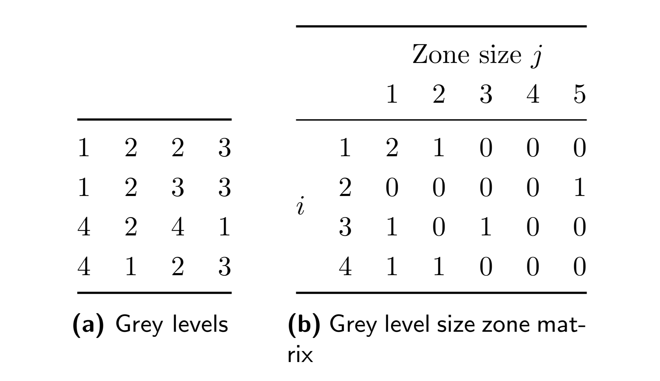
Fig. 15 Original image with grey levels (a); and corresponding grey level size zone matrix (GLSZM) under 8-connectedness (b). Element \(s_{i,j}\) of the GLSZM indicates the number of times a zone of \(j\) linked pixels and grey level \(i\) occurs within the image.

Aggregating features

Three methods can be used to aggregate GLSZMs and arrive at a single feature value. A schematic example is shown in Fig. 16. A feature may be aggregated as follows:

1. Features are computed from 2D matrices and averaged over slices (8QNN).
2. The feature is computed from a single matrix after merging all 2D matrices (62GR).
3. The feature is computed from a 3D matrix (KOBO).

Method 2 involves merging GLSZMs by summing the number of zones \(s_{ij}\) over the GLSZM for the different slices. Note that when matrices are merged, \(N_v\) should likewise be summed to retain consistency. Feature values may dependent strongly on the aggregation method.

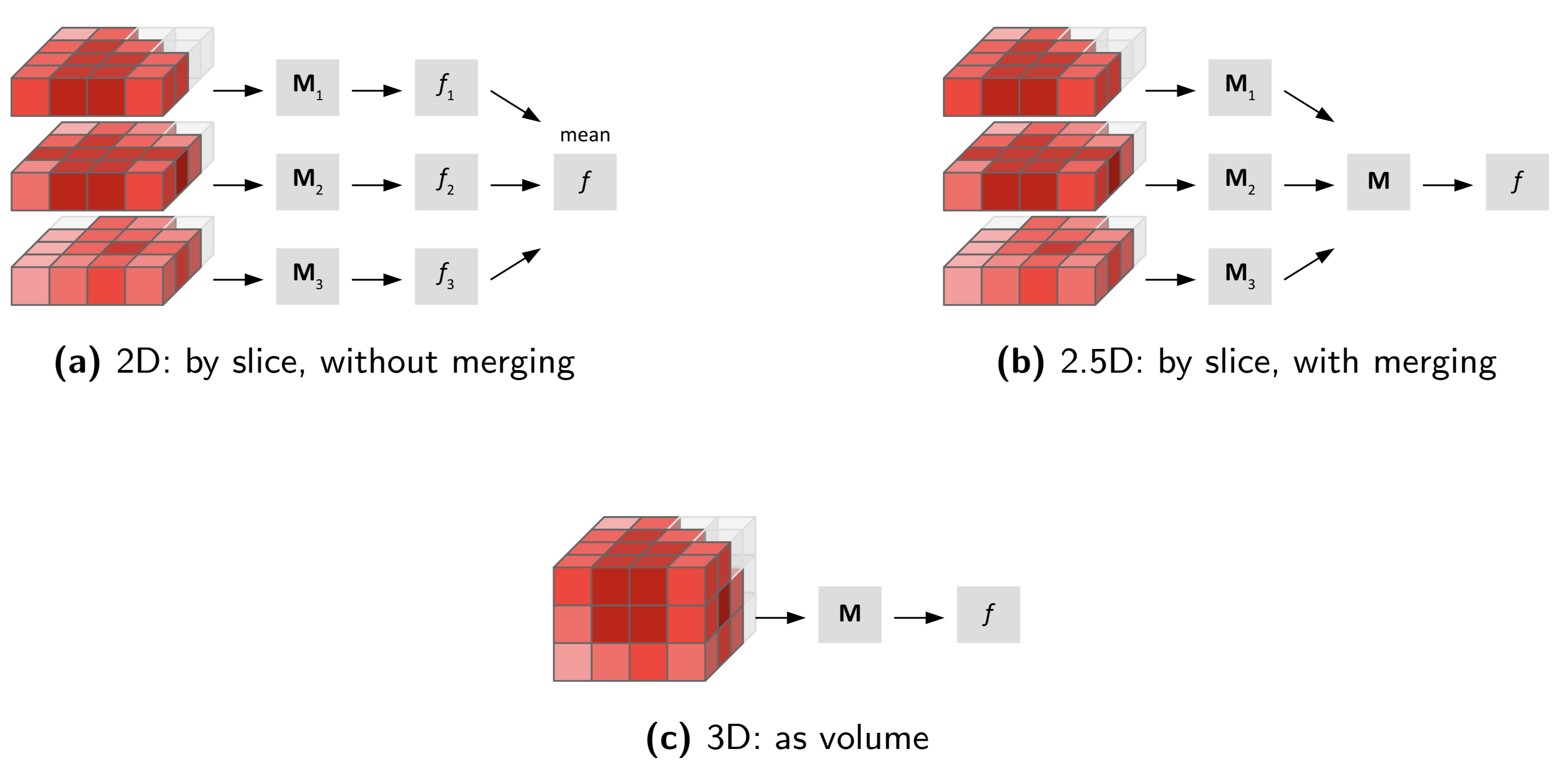
Fig. 16 Approaches to calculating grey level size zone matrix-based features. \(\mathbf{M}_{k}\) are texture matrices calculated for slice \(k\) (if applicable), and \(f_{k}\) is the corresponding feature value. In (b) the matrices from the different slices are merged prior to feature calculation.

Distances

The default neighbourhood for GLSZM is constructed using Chebyshev distance \(\delta=1\). Manhattan or Euclidean norms may also be used to construct a neighbourhood, and both lead to a 6-connected (3D) and 4-connected (2D) neighbourhoods. Larger distances are also technically possible, but will occasionally cause separate zones with the same intensity to be considered as belonging to the same zone. Using different neighbourhoods for determining voxel linkage is non-standard use, and we caution against it due to potential reproducibility issues.

Note on feature references

GLSZM feature definitions are based on the definitions of GLRLM features [Thibault2014]. Hence, references may be found in the section on GLRLM (Grey level run length based features).

Small zone emphasis

This feature emphasises small zones. It is defined as:

\[F_{\mathit{szm.sze}} = \frac{1}{N_s} \sum_{j=1}^{N_z} \frac{s_{.j}}{j^2}\]

data	aggr. method	value	tol.	consensus
dig. phantom	2D	0.363	—	strong
dig. phantom	2.5D	0.368	—	strong
dig. phantom	3D	0.255	—	very strong
config. A	2D	0.688	0.003	strong
config. A	2.5D	0.68	0.003	strong
config. B	2D	0.745	0.003	strong
config. B	2.5D	0.741	0.003	strong
config. C	3D	0.695	0.001	strong
config. D	3D	0.637	0.005	strong
config. E	3D	0.676	0.003	strong

Large zone emphasis

48P8

This feature emphasises large zones. It is defined as:

\[F_{\mathit{szm.lze}} = \frac{1}{N_s} \sum_{j=1}^{N_z} j^2 s_{.j}\]

data	aggr. method	value	tol.	consensus
dig. phantom	2D	43.9	—	strong
dig. phantom	2.5D	34.2	—	strong
dig. phantom	3D	550	—	very strong
config. A	2D	625	9	strong
config. A	2.5D	675	8	strong
config. B	2D	439	8	strong
config. B	2.5D	444	8	strong
config. C	3D	\(3.89 \times 10^{4}\)	900	strong
config. D	3D	\(9.91 \times 10^{4}\)	\(2.8 \times 10^{3}\)	strong
config. E	3D	\(5.86 \times 10^{4}\)	800	strong

Low grey level zone emphasis

XMSY

This feature is a grey level analogue to small zone emphasis. Instead of small zone sizes, low grey levels are emphasised. The feature is defined as:

\[F_{\mathit{szm.lgze}}=\frac{1}{N_s} \sum_{i=1}^{N_g} \frac{s_{i.}}{i^2}\]

data	aggr. method	value	tol.	consensus
dig. phantom	2D	0.371	—	strong
dig. phantom	2.5D	0.368	—	strong
dig. phantom	3D	0.253	—	very strong
config. A	2D	0.0368	0.0005	strong
config. A	2.5D	0.0291	0.0005	strong
config. B	2D	0.0475	0.001	strong
config. B	2.5D	0.0387	0.001	strong
config. C	3D	0.00235	\(6 \times 10^{-5}\)	strong
config. D	3D	0.0409	0.0005	strong
config. E	3D	0.034	0.0004	strong

High grey level zone emphasis

5GN9

The high grey level zone emphasis feature is a grey level analogue to large zone emphasis. The feature emphasises high grey levels, and is defined as:

\[F_{\mathit{szm.hgze}}=\frac{1}{N_s} \sum_{i=1}^{N_g} i^2 s_{i.}\]

data	aggr. method	value	tol.	consensus
dig. phantom	2D	16.4	—	strong
dig. phantom	2.5D	16.2	—	strong
dig. phantom	3D	15.6	—	very strong
config. A	2D	363	3	strong
config. A	2.5D	370	3	strong
config. B	2D	284	11	strong
config. B	2.5D	284	11	strong
config. C	3D	971	7	strong
config. D	3D	188	10	strong
config. E	3D	286	6	strong

Small zone low grey level emphasis

5RAI

This feature emphasises zone counts within the upper left quadrant of the GLSZM, where small zone sizes and low grey levels are located. It is defined as:

\[F_{\mathit{szm.szlge}}=\frac{1}{N_s} \sum_{i=1}^{N_g} \sum_{j=1}^{N_z} \frac{s_{ij}}{i^2 j^2}\]

data	aggr. method	value	tol.	consensus
dig. phantom	2D	0.0259	—	strong
dig. phantom	2.5D	0.0295	—	strong
dig. phantom	3D	0.0256	—	very strong
config. A	2D	0.0298	0.0005	strong
config. A	2.5D	0.0237	0.0005	strong
config. B	2D	0.0415	0.0008	strong
config. B	2.5D	0.0335	0.0009	strong
config. C	3D	0.0016	\(4 \times 10^{-5}\)	strong
config. D	3D	0.0248	0.0004	strong
config. E	3D	0.0224	0.0004	strong

Small zone high grey level emphasis

HW1V

This feature emphasises zone counts in the lower left quadrant of the GLSZM, where small zone sizes and high grey levels are located. The feature is defined as:

\[F_{\mathit{szm.szhge}}=\frac{1}{N_s} \sum_{i=1}^{N_g} \sum_{j=1}^{N_z} \frac{i^2 s_{ij}}{j^2}\]

data	aggr. method	value	tol.	consensus
dig. phantom	2D	10.3	—	strong
dig. phantom	2.5D	9.87	—	strong
dig. phantom	3D	2.76	—	very strong
config. A	2D	226	1	strong
config. A	2.5D	229	1	strong
config. B	2D	190	7	strong
config. B	2.5D	190	7	strong
config. C	3D	657	4	strong
config. D	3D	117	7	strong
config. E	3D	186	4	strong

Large zone low grey level emphasis

YH51

This feature emphasises zone counts in the upper right quadrant of the GLSZM, where large zone sizes and low grey levels are located. The feature is defined as:

\[F_{\mathit{szm.lzlge}}=\frac{1}{N_s} \sum_{i=1}^{N_g} \sum_{j=1}^{N_z} \frac{j^2 s_{ij}}{i^2}\]

data	aggr. method	value	tol.	consensus
dig. phantom	2D	40.4	—	strong
dig. phantom	2.5D	30.6	—	strong
dig. phantom	3D	503	—	very strong
config. A	2D	1.35	0.03	strong
config. A	2.5D	1.44	0.02	strong
config. B	2D	1.15	0.04	strong
config. B	2.5D	1.16	0.04	strong
config. C	3D	21.6	0.5	strong
config. D	3D	241	14	strong
config. E	3D	105	4	strong

Large zone high grey level emphasis

J17V

This feature emphasises zone counts in the lower right quadrant of the GLSZM, where large zone sizes and high grey levels are located. The feature is defined as:

\[F_{\mathit{szm.lzhge}}=\frac{1}{N_s} \sum_{i=1}^{N_g} \sum_{j=1}^{N_z} i^2 j^2 s_{ij}\]

data	aggr. method	value	tol.	consensus
dig. phantom	2D	113	—	strong
dig. phantom	2.5D	107	—	strong
dig. phantom	3D	\(1.49 \times 10^{3}\)	—	very strong
config. A	2D	\(3.16 \times 10^{5}\)	\(5 \times 10^{3}\)	strong
config. A	2.5D	\(3.38 \times 10^{5}\)	\(5 \times 10^{3}\)	strong
config. B	2D	\(1.81 \times 10^{5}\)	\(3 \times 10^{3}\)	strong
config. B	2.5D	\(1.81 \times 10^{5}\)	\(3 \times 10^{3}\)	strong
config. C	3D	\(7.07 \times 10^{7}\)	\(1.5 \times 10^{6}\)	strong
config. D	3D	\(4.14 \times 10^{7}\)	\(3 \times 10^{5}\)	strong
config. E	3D	\(3.36 \times 10^{7}\)	\(3 \times 10^{5}\)	strong

Grey level non-uniformity

JNSA

This feature assesses the distribution of zone counts over the grey values. The feature value is low when zone counts are equally distributed along grey levels. The feature is defined as:

\[F_{\mathit{szm.glnu}}= \frac{1}{N_s} \sum_{i=1}^{N_g} s_{i.}^2\]

data	aggr. method	value	tol.	consensus
dig. phantom	2D	1.41	—	strong
dig. phantom	2.5D	5.44	—	strong
dig. phantom	3D	1.4	—	very strong
config. A	2D	82.2	0.1	strong
config. A	2.5D	\(1.8 \times 10^{3}\)	10	strong
config. B	2D	20.5	0.1	strong
config. B	2.5D	437	3	strong
config. C	3D	195	6	strong
config. D	3D	212	6	very strong
config. E	3D	231	6	strong

Normalised grey level non-uniformity

Y1RO

This is a normalised version of the grey level non-uniformity feature. It is defined as:

\[F_{\mathit{szm.glnu.norm}}= \frac{1}{N_s^2} \sum_{i=1}^{N_g} s_{i.}^2\]

data	aggr. method	value	tol.	consensus
dig. phantom	2D	0.323	—	strong
dig. phantom	2.5D	0.302	—	strong
dig. phantom	3D	0.28	—	very strong
config. A	2D	0.0728	0.0014	strong
config. A	2.5D	0.0622	0.0007	strong
config. B	2D	0.0789	0.001	strong
config. B	2.5D	0.0613	0.0005	strong
config. C	3D	0.0286	0.0003	strong
config. D	3D	0.0491	0.0008	strong
config. E	3D	0.0414	0.0003	strong

Zone size non-uniformity

4JP3

This features assesses the distribution of zone counts over the different zone sizes. Zone size non-uniformity is low when zone counts are equally distributed along zone sizes. It is defined as:

\[F_{\mathit{szm.zsnu}}= \frac{1}{N_s} \sum_{j=1}^{N_z} s_{.j}^2\]

data	aggr. method	value	tol.	consensus
dig. phantom	2D	1.49	—	strong
dig. phantom	2.5D	3.44	—	strong
dig. phantom	3D	1	—	very strong
config. A	2D	479	4	strong
config. A	2.5D	\(1.24 \times 10^{4}\)	100	strong
config. B	2D	140	3	strong
config. B	2.5D	\(3.63 \times 10^{3}\)	70	strong
config. C	3D	\(3.04 \times 10^{3}\)	100	strong
config. D	3D	\(1.63 \times 10^{3}\)	10	strong
config. E	3D	\(2.37 \times 10^{3}\)	40	strong

Normalised zone size non-uniformity

VB3A

This is a normalised version of zone size non-uniformity. It is defined as:

\[F_{\mathit{szm.zsnu.norm}}= \frac{1}{N_s^2} \sum_{i=1}^{N_z} s_{.j}^2\]

data	aggr. method	value	tol.	consensus
dig. phantom	2D	0.333	—	strong
dig. phantom	2.5D	0.191	—	strong
dig. phantom	3D	0.2	—	very strong
config. A	2D	0.44	0.004	strong
config. A	2.5D	0.427	0.004	strong
config. B	2D	0.521	0.004	strong
config. B	2.5D	0.509	0.004	strong
config. C	3D	0.447	0.001	strong
config. D	3D	0.377	0.006	strong
config. E	3D	0.424	0.004	strong

Zone percentage

P30P

This feature measures the fraction of the number of realised zones and the maximum number of potential zones. Highly uniform ROIs produce a low zone percentage. It is defined as:

\[F_{\mathit{szm.z.perc}}=\frac{N_s}{N_v}\]

data	aggr. method	value	tol.	consensus
dig. phantom	2D	0.24	—	strong
dig. phantom	2.5D	0.243	—	strong
dig. phantom	3D	0.0676	—	very strong
config. A	2D	0.3	0.003	strong
config. A	2.5D	0.253	0.004	strong
config. B	2D	0.324	0.001	strong
config. B	2.5D	0.26	0.002	strong
config. C	3D	0.148	0.003	strong
config. D	3D	0.0972	0.0007	strong
config. E	3D	0.126	0.001	strong

Grey level variance

BYLV

This feature estimates the variance in zone counts over the grey levels. Let \(p_{ij} = s_{ij}/N_s\) be the joint probability estimate for finding zones with discretised grey level \(i\) and size \(j\). The feature is then defined as:

\[F_{\mathit{szm.gl.var}}= \sum_{i=1}^{N_g} \sum_{j=1}^{N_z} (i-\mu)^2 p_{ij}\]

Here, \(\mu = \sum_{i=1}^{N_g} \sum_{j=1}^{N_z} i\,p_{ij}\).

data	aggr. method	value	tol.	consensus
dig. phantom	2D	3.97	—	strong
dig. phantom	2.5D	3.92	—	strong
dig. phantom	3D	2.64	—	very strong
config. A	2D	42.7	0.7	strong
config. A	2.5D	47.9	0.4	strong
config. B	2D	36.1	0.3	strong
config. B	2.5D	41	0.7	strong
config. C	3D	106	1	strong
config. D	3D	32.7	1.6	strong
config. E	3D	50.8	0.9	strong

Zone size variance

3NSA

This feature estimates the variance in zone counts over the different zone sizes. As before let \(p_{ij} = s_{ij}/N_s\). The feature is defined as:

\[F_{\mathit{szm.zs.var}}= \sum_{i=1}^{N_g} \sum_{j=1}^{N_z} (j-\mu)^2 p_{ij}\]

Mean zone size is defined as \(\mu = \sum_{i=1}^{N_g} \sum_{j=1}^{N_z} j\,p_{ij}\).

data	aggr. method	value	tol.	consensus
dig. phantom	2D	21	—	strong
dig. phantom	2.5D	17.3	—	strong
dig. phantom	3D	331	—	very strong
config. A	2D	609	9	strong
config. A	2.5D	660	8	strong
config. B	2D	423	8	strong
config. B	2.5D	429	8	strong
config. C	3D	\(3.89 \times 10^{4}\)	900	strong
config. D	3D	\(9.9 \times 10^{4}\)	\(2.8 \times 10^{3}\)	strong
config. E	3D	\(5.85 \times 10^{4}\)	800	strong

Zone size entropy

GU8N

Let \(p_{ij} = s_{ij}/N_s\). Zone size entropy is then defined as:

\[F_{\mathit{szm.zs.entr}} = - \sum_{i=1}^{N_g} \sum_{j=1}^{N_z} p_{ij} \log_2 p_{ij}\]

data	aggr. method	value	tol.	consensus
dig. phantom	2D	1.93	—	strong
dig. phantom	2.5D	3.08	—	strong
dig. phantom	3D	2.32	—	very strong
config. A	2D	5.92	0.02	strong
config. A	2.5D	6.39	0.01	strong
config. B	2D	5.29	0.01	strong
config. B	2.5D	5.98	0.02	strong
config. C	3D	7	0.01	strong
config. D	3D	6.52	0.01	strong
config. E	3D	6.57	0.01	strong

Grey level distance zone based features

VMDZ

The grey level distance zone matrix (GLDZM) counts the number of groups (or zones) of linked voxels which share a specific discretised grey level value and possess the same distance to ROI edge [Thibault2014]. The GLDZM thus captures the relation between location and grey level. Two maps are required to calculate the GLDZM. The first is a grey level zone map, which is identical to the one created for the grey level size zone matrix (GLSZM), see Grey level size zone based features. The second is a distance map, which will be described in detail later.

As with GSLZM, neighbouring voxels are linked if they share the same grey level value. Whether a voxel classifies as a neighbour depends on its connectedness. We consider 26-connectedness for a 3D approach and 8-connectedness in the 2D approach.

The distance to the ROI edge is defined according to 6 and 4-connectedness for 3D and 2D, respectively. Because of the connectedness definition used, the distance of a voxel to the outer border is equal to the minimum number edges of neighbouring voxels that need to be crossed to reach the ROI edge. The distance for a linked group of voxels with the same grey value is equal to the minimum distance for the respective voxels in the distance map.

Our definition deviates from the original by [Thibault2014]. The original was defined in a rectangular 2D image, whereas ROIs are rarely rectangular cuboids. Approximating distance using Chamfer maps is then no longer a fast and easy solution. Determining distance iteratively in 6 or 4-connectedness is a relatively efficient solution, implemented as follows:

1. The ROI mask is morphologically eroded using the appropriate (6 or 4-connected) structure element.
2. All eroded ROI voxels are updated in the distance map by adding 1.
3. The above steps are performed iteratively until the ROI mask is empty.

A second difference with the original definition is that the lowest possible distance is \(1\) instead of \(0\) for voxels directly on the ROI edge. This prevents division by \(0\) for some features.

Let \(\mathbf{M}\) be the \(N_g \times N_d\) grey level size zone matrix, where \(N_g\) is the number of discretised grey levels present in the ROI intensity mask and \(N_d\) the largest distance of any zone. Element \(d_{ij}=d(i,j)\) of \(\mathbf{M}\) is then number of zones with discretised grey level \(i\) and distance \(j\). Furthermore, let \(N_v\) be the number of voxels and \(N_s=\sum_{i=1}^{N_g}\sum_{j=1}^{N_d}d_{ij}\) be the total zone count. Marginal sums can likewise be defined. Let \(d_{i.}=\sum_{j=1}^{N_d}d_{ij}\) be the number of zones with discretised grey level \(i\), regardless of distance. Likewise, let \(d_{.j}=\sum_{i=1}^{N_g}d_{ij}\) be the number of zones with distance \(j\), regardless of grey level. A two dimensional example is shown in Fig. 17.

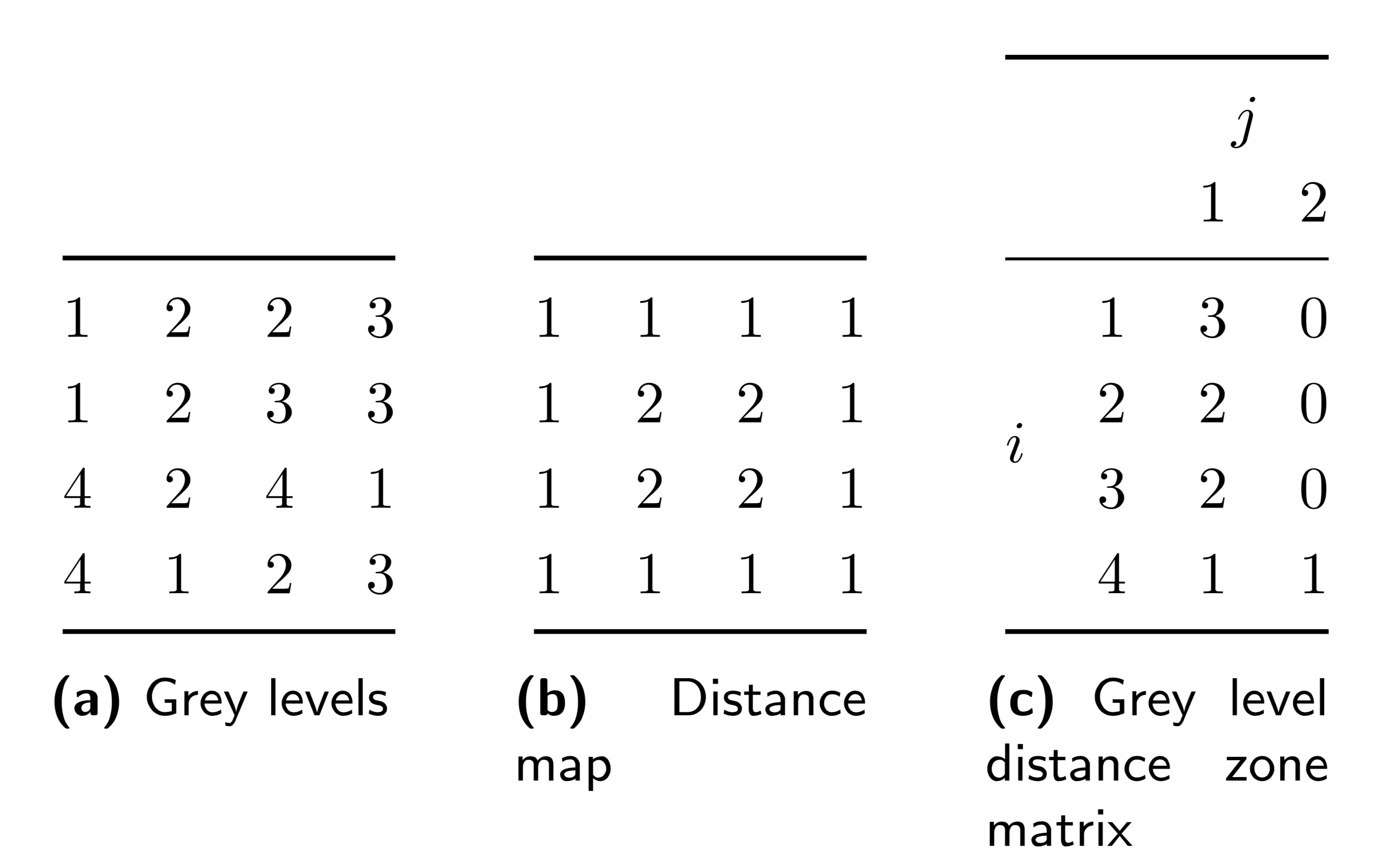
Fig. 17 Original image with grey levels (a); corresponding distance map for distance to border (b); and corresponding grey level distance zone matrix (GLDZM) under 4-connectedness (c). Element \(d_{i,j}\) of the GLDZM indicates the number of times a zone with grey level \(i\) and a minimum distance to border \(j\) occurs within the image.

Morphological and intensity masks.

The GLDZM is special in that it uses both ROI masks. The distance map is determined using the morphological ROI mask, whereas the intensity mask is used for determining the zones, as with the GLSZM.

Aggregating features

Three methods can be used to aggregate GLDZMs and arrive at a single feature value. A schematic example was previously shown in Figure Fig. 16. A feature may be aggregated as follows:

1. Features are computed from 2D matrices and averaged over slices (8QNN).
2. The feature is computed from a single matrix after merging all 2D matrices (62GR).
3. The feature is computed from a 3D matrix (KOBO).

Method 2 involves merging GLDZMs by summing the number of zones \(d_{ij}\) over the GLDZM for the different slices. Note that when matrices are merged, \(N_v\) should likewise be summed to retain consistency. Feature values may dependent strongly on the aggregation method.

Distances

In addition to the use of different distance norms to determine voxel linkage, as described in Grey level size zone based features, different distance norms may be used to determine distance of zones to the boundary. The default is to use the Manhattan norm which allows for a computationally efficient implementation, as described above. A similar implementation is possible using the Chebyshev norm, as it merely changes connectedness of the structure element. Implementations using an Euclidean distance norm are less efficient as this demands searching for the nearest non-ROI voxel for each of the \(N_v\) voxels in the ROI. An added issue is that Euclidean norms may lead to a wide range of different distances \(j\) that require rounding before constructing the grey level distance zone matrix \(\mathbf{M}\). Using different distance norms is non-standard use, and we caution against it due to potential reproducibility issues.

Note on feature references

GLDZM feature definitions are based on the definitions of GLRLM features [Thibault2014]. Hence, references may be found in the section on GLRLM (Grey level run length based features).

Small distance emphasis

0GBI

This feature emphasises small distances. It is defined as:

\[F_{\mathit{dzm.sde}} = \frac{1}{N_s} \sum_{j=1}^{N_d} \frac{d_{.j}}{j^2}\]

data	aggr. method	value	tol.	consensus
dig. phantom	2D	0.946	—	strong
dig. phantom	2.5D	0.917	—	moderate
dig. phantom	3D	1	—	very strong
config. A	2D	0.192	0.006	strong
config. A	2.5D	0.168	0.005	strong
config. B	2D	0.36	0.005	strong
config. B	2.5D	0.329	0.004	strong
config. C	3D	0.531	0.006	strong
config. D	3D	0.579	0.004	strong
config. E	3D	0.527	0.004	moderate

Large distance emphasis

MB4I

This feature emphasises large distances. It is defined as:

\[F_{\mathit{dzm.lde}} = \frac{1}{N_s} \sum_{j=1}^{N_d} j^2 d_{.j}\]

data	aggr. method	value	tol.	consensus
dig. phantom	2D	1.21	—	strong
dig. phantom	2.5D	1.33	—	moderate
dig. phantom	3D	1	—	very strong
config. A	2D	161	1	moderate
config. A	2.5D	178	1	moderate
config. B	2D	31.6	0.2	moderate
config. B	2.5D	34.3	0.2	moderate
config. C	3D	11	0.3	strong
config. D	3D	10.3	0.1	strong
config. E	3D	12.6	0.1	moderate

Low grey level zone emphasis

S1RA

This feature is a grey level analogue to small distance emphasis. Instead of small zone distances, low grey levels are emphasised. The feature is defined as:

\[F_{\mathit{dzm.lgze}}=\frac{1}{N_s} \sum_{i=1}^{N_g} \frac{d_{i.}}{i^2}\]

data	aggr. method	value	tol.	consensus
dig. phantom	2D	0.371	—	strong
dig. phantom	2.5D	0.368	—	moderate
dig. phantom	3D	0.253	—	very strong
config. A	2D	0.0368	0.0005	strong
config. A	2.5D	0.0291	0.0005	strong
config. B	2D	0.0475	0.001	strong
config. B	2.5D	0.0387	0.001	strong
config. C	3D	0.00235	\(6 \times 10^{-5}\)	strong
config. D	3D	0.0409	0.0005	strong
config. E	3D	0.034	0.0004	moderate

High grey level zone emphasis

K26C

The high grey level zone emphasis feature is a grey level analogue to large distance emphasis. The feature emphasises high grey levels, and is defined as:

\[F_{\mathit{dzm.hgze}}=\frac{1}{N_s} \sum_{i=1}^{N_g} i^2 d_{i.}\]

data	aggr. method	value	tol.	consensus
dig. phantom	2D	16.4	—	strong
dig. phantom	2.5D	16.2	—	moderate
dig. phantom	3D	15.6	—	very strong
config. A	2D	363	3	strong
config. A	2.5D	370	3	strong
config. B	2D	284	11	strong
config. B	2.5D	284	11	strong
config. C	3D	971	7	strong
config. D	3D	188	10	strong
config. E	3D	286	6	strong

Small distance low grey level emphasis

RUVG

This feature emphasises runs in the upper left quadrant of the GLDZM, where small zone distances and low grey levels are located. It is defined as:

\[F_{\mathit{dzm.sdlge}}=\frac{1}{N_s} \sum_{i=1}^{N_g} \sum_{j=1}^{N_d} \frac{d_{ij}}{i^2 j^2}\]

data	aggr. method	value	tol.	consensus
dig. phantom	2D	0.367	—	strong
dig. phantom	2.5D	0.362	—	moderate
dig. phantom	3D	0.253	—	very strong
config. A	2D	0.00913	0.00023	strong
config. A	2.5D	0.00788	0.00022	strong
config. B	2D	0.0192	0.0005	strong
config. B	2.5D	0.0168	0.0005	strong
config. C	3D	0.00149	\(4 \times 10^{-5}\)	strong
config. D	3D	0.0302	0.0006	strong
config. E	3D	0.0228	0.0003	moderate

Small distance high grey level emphasis

DKNJ

This feature emphasises runs in the lower left quadrant of the GLDZM, where small zone distances and high grey levels are located. Small distance high grey level emphasis is defined as:

\[F_{\mathit{dzm.sdhge}}=\frac{1}{N_s} \sum_{i=1}^{N_g} \sum_{j=1}^{N_d} \frac{i^2 d_{ij}}{j^2}\]

data	aggr. method	value	tol.	consensus
dig. phantom	2D	15.2	—	strong
dig. phantom	2.5D	14.3	—	moderate
dig. phantom	3D	15.6	—	very strong
config. A	2D	60.1	3.3	strong
config. A	2.5D	49.5	2.8	strong
config. B	2D	95.7	5.5	strong
config. B	2.5D	81.4	4.6	strong
config. C	3D	476	11	strong
config. D	3D	99.3	5.1	strong
config. E	3D	136	4	moderate

Large distance low grey level emphasis

A7WM

This feature emphasises runs in the upper right quadrant of the GLDZM, where large zone distances and low grey levels are located. The feature is defined as:

\[F_{\mathit{dzm.ldlge}}=\frac{1}{N_s} \sum_{i=1}^{N_g} \sum_{j=1}^{N_d} \frac{j^2 d_{ij}}{i^2}\]

data	aggr. method	value	tol.	consensus
dig. phantom	2D	0.386	—	strong
dig. phantom	2.5D	0.391	—	moderate
dig. phantom	3D	0.253	—	very strong
config. A	2D	2.96	0.02	moderate
config. A	2.5D	2.31	0.01	moderate
config. B	2D	0.934	0.018	moderate
config. B	2.5D	0.748	0.017	moderate
config. C	3D	0.0154	0.0005	strong
config. D	3D	0.183	0.004	strong
config. E	3D	0.179	0.004	moderate

Large distance high grey level emphasis

KLTH

This feature emphasises runs in the lower right quadrant of the GLDZM, where large zone distances and high grey levels are located. The large distance high grey level emphasis feature is defined as:

\[F_{\mathit{dzm.ldhge}}=\frac{1}{N_s} \sum_{i=1}^{N_g} \sum_{j=1}^{N_d} i^2 j^2 d_{ij}\]

data	aggr. method	value	tol.	consensus
dig. phantom	2D	21.3	—	strong
dig. phantom	2.5D	23.7	—	moderate
dig. phantom	3D	15.6	—	very strong
config. A	2D	\(7.01 \times 10^{4}\)	100	moderate
config. A	2.5D	\(7.95 \times 10^{4}\)	100	moderate
config. B	2D	\(1.06 \times 10^{4}\)	300	strong
config. B	2.5D	\(1.16 \times 10^{4}\)	400	strong
config. C	3D	\(1.34 \times 10^{4}\)	200	strong
config. D	3D	\(2.62 \times 10^{3}\)	110	strong
config. E	3D	\(4.85 \times 10^{3}\)	60	moderate

Grey level non-uniformity

VFT7

This feature measures the distribution of zone counts over the grey values. Grey level non-uniformity is low when zone counts are equally distributed along grey levels. The feature is defined as:

\[F_{\mathit{dzm.glnu}}= \frac{1}{N_s} \sum_{i=1}^{N_g} d_{i.}^2\]

data	aggr. method	value	tol.	consensus
dig. phantom	2D	1.41	—	strong
dig. phantom	2.5D	5.44	—	moderate
dig. phantom	3D	1.4	—	very strong
config. A	2D	82.2	0.1	strong
config. A	2.5D	\(1.8 \times 10^{3}\)	10	strong
config. B	2D	20.5	0.1	strong
config. B	2.5D	437	3	strong
config. C	3D	195	6	strong
config. D	3D	212	6	strong
config. E	3D	231	6	moderate

Normalised grey level non-uniformity

7HP3

This is a normalised version of the grey level non-uniformity feature. It is defined as:

\[F_{\mathit{dzm.glnu.norm}}= \frac{1}{N_s^2} \sum_{i=1}^{N_g} d_{i.}^2\]

data	aggr. method	value	tol.	consensus
dig. phantom	2D	0.323	—	strong
dig. phantom	2.5D	0.302	—	moderate
dig. phantom	3D	0.28	—	very strong
config. A	2D	0.0728	0.0014	strong
config. A	2.5D	0.0622	0.0007	strong
config. B	2D	0.0789	0.001	strong
config. B	2.5D	0.0613	0.0005	strong
config. C	3D	0.0286	0.0003	strong
config. D	3D	0.0491	0.0008	strong
config. E	3D	0.0414	0.0003	moderate

Zone distance non-uniformity

V294

Zone distance non-uniformity measures the distribution of zone counts over the different zone distances. Zone distance non-uniformity is low when zone counts are equally distributed along zone distances. It is defined as:

\[F_{\mathit{dzm.zdnu}}= \frac{1}{N_s} \sum_{j=1}^{N_d} d_{.j}^2\]

data	aggr. method	value	tol.	consensus
dig. phantom	2D	3.79	—	strong
dig. phantom	2.5D	14.4	—	moderate
dig. phantom	3D	5	—	very strong
config. A	2D	64	0.4	moderate
config. A	2.5D	\(1.57 \times 10^{3}\)	10	strong
config. B	2D	39.8	0.3	moderate
config. B	2.5D	963	6	moderate
config. C	3D	\(1.87 \times 10^{3}\)	40	strong
config. D	3D	\(1.37 \times 10^{3}\)	20	strong
config. E	3D	\(1.5 \times 10^{3}\)	30	moderate

Normalised zone distance non-uniformity

IATH

This is a normalised version of the zone distance non-uniformity feature. It is defined as:

\[F_{\mathit{dzm.zdnu.norm}}= \frac{1}{N_s^2} \sum_{i=1}^{N_d} d_{.j}^2\]

data	aggr. method	value	tol.	consensus
dig. phantom	2D	0.898	—	strong
dig. phantom	2.5D	0.802	—	moderate
dig. phantom	3D	1	—	very strong
config. A	2D	0.0716	0.0022	strong
config. A	2.5D	0.0543	0.0014	strong
config. B	2D	0.174	0.003	strong
config. B	2.5D	0.135	0.001	strong
config. C	3D	0.274	0.005	strong
config. D	3D	0.317	0.004	strong
config. E	3D	0.269	0.003	moderate

Zone percentage

VIWW

This feature measures the fraction of the number of realised zones and the maximum number of potential zones. Highly uniform ROIs produce a low zone percentage. It is defined as:

\[F_{\mathit{dzm.z.perc}}=\frac{N_s}{N_v}\]

data	aggr. method	value	tol.	consensus
dig. phantom	2D	0.24	—	strong
dig. phantom	2.5D	0.243	—	moderate
dig. phantom	3D	0.0676	—	very strong
config. A	2D	0.3	0.003	strong
config. A	2.5D	0.253	0.004	moderate
config. B	2D	0.324	0.001	strong
config. B	2.5D	0.26	0.002	moderate
config. C	3D	0.148	0.003	strong
config. D	3D	0.0972	0.0007	strong
config. E	3D	0.126	0.001	moderate

Grey level variance

QK93

This feature estimates the variance in zone counts over the grey levels. Let \(p_{ij} = d_{ij}/N_s\) be the joint probability estimate for finding zones with discretised grey level \(i\) at distance \(j\). The feature is then defined as:

\[F_{\mathit{dzm.gl.var}}= \sum_{i=1}^{N_g} \sum_{j=1}^{N_d} (i-\mu)^2 p_{ij}\]

Here, \(\mu = \sum_{i=1}^{N_g} \sum_{j=1}^{N_d} i\,p_{ij}\).

data	aggr. method	value	tol.	consensus
dig. phantom	2D	3.97	—	strong
dig. phantom	2.5D	3.92	—	moderate
dig. phantom	3D	2.64	—	very strong
config. A	2D	42.7	0.7	moderate
config. A	2.5D	47.9	0.4	strong
config. B	2D	36.1	0.3	moderate
config. B	2.5D	41	0.7	strong
config. C	3D	106	1	strong
config. D	3D	32.7	1.6	strong
config. E	3D	50.8	0.9	strong

Zone distance variance

7WT1

This feature estimates the variance in zone counts for the different zone distances. As before let \(p_{ij} = d_{ij}/N_s\). The feature is defined as:

\[F_{\mathit{dzm.zd.var}}= \sum_{i=1}^{N_g} \sum_{j=1}^{N_d} (j-\mu)^2 p_{ij}\]

Mean zone size is defined as \(\mu = \sum_{i=1}^{N_g} \sum_{j=1}^{N_d} j\,p_{ij}\).

data	aggr. method	value	tol.	consensus
dig. phantom	2D	0.051	—	strong
dig. phantom	2.5D	0.0988	—	moderate
dig. phantom	3D	0	—	very strong
config. A	2D	69.4	0.1	moderate
config. A	2.5D	78.9	0.1	moderate
config. B	2D	13.5	0.1	moderate
config. B	2.5D	15	0.1	moderate
config. C	3D	4.6	0.06	strong
config. D	3D	4.61	0.04	strong
config. E	3D	5.56	0.05	strong

Zone distance entropy

GBDU

Again, let \(p_{ij} = d_{ij}/N_s\). Zone distance entropy is then defined as:

\[F_{\mathit{dzm.zd.entr}} = - \sum_{i=1}^{N_g} \sum_{j=1}^{N_d} p_{ij} \log_2 p_{ij}\]

data	aggr. method	value	tol.	consensus
dig. phantom	2D	1.73	—	strong
dig. phantom	2.5D	2	—	moderate
dig. phantom	3D	1.92	—	very strong
config. A	2D	8	0.04	strong
config. A	2.5D	8.87	0.03	strong
config. B	2D	6.47	0.03	strong
config. B	2.5D	7.58	0.01	moderate
config. C	3D	7.56	0.03	strong
config. D	3D	6.61	0.03	strong
config. E	3D	7.06	0.01	moderate

Neighbourhood grey tone difference based features

IPET

[Amadasun1989] introduced an alternative to the grey level co-occurrence matrix. The neighbourhood grey tone difference matrix (NGTDM) contains the sum of grey level differences of pixels/voxels with discretised grey level \(i\) and the average discretised grey level of neighbouring pixels/voxels within a Chebyshev distance \(\delta\). For 3D volumes, we can extend the original definition by Amadasun and King. Let \(X_{d,k}\) be the discretised grey level of a voxel at position \(\mathbf{k}=(k_x,k_y,k_z)\). Then the average grey level within a neighbourhood centred at \((k_x,k_y,k_z)\), but excluding \((k_x,k_y,k_z)\) itself is:

\[\begin{split}\begin{aligned} \overline{X}_k& =\frac{1}{W}\sum_{m_z{=}-\delta}^\delta \sum_{m_y{=}-\delta}^\delta \sum_{m_x{=}-\delta}^\delta X_{d}(k_x{+}m_x, k_y{+}m_y, k_z{+}m_z)\\ & \hspace{6cm} (m_x,m_y,m_z)\neq (0,0,0)\end{aligned}\end{split}\]

\(W=(2\delta+1)^3-1\) is the size of the 3D neighbourhood. For 2D \(W=(2\delta+1)^2-1\), and averages are not calculated between different slices. Neighbourhood grey tone difference \(s_i\) for discretised grey level \(i\) is then:

\[s_i=\sum_{k}^{N_v} |i-\overline{X}_k| \, \big[X_d(\mathbf{k})=i \text{ and } k \text{ has a valid neighbourhood}\big]\]

Here, \([\ldots]\) is an Iverson bracket, which is \(1\) if the conditions that the grey level \(X_{d,k}\) of voxel \(k\) is equal to \(i\) and the voxel has a valid neighbourhood are both true; it is \(0\) otherwise. \(N_v\) is the number of voxels in the ROI intensity mask.

A 2D example is shown in Fig. 18. A distance of \(\delta=1\) is used in this example, leading to 8 neighbouring pixels. Entry \(s_1=0\) because there are no valid pixels with grey level \(1\). Two pixels have grey level \(2\). The average value of their neighbours are \(19/8\) and \(21/8\). Thus \(s_2=|2-19/8|+|2-21/8|=1\). Similarly \(s_3=|3-19/8|=0.625\) and \(s_4=|4-17/8|=1.825\).

We deviate from the original definition by [Amadasun1989] as we do not demand that valid neighbourhoods are completely inside the ROI. In an irregular ROI mask, valid neighbourhoods may simply not exist for a distance \(\delta\). Instead, we consider a valid neighbourhood to exist if there is at least one neighbouring voxel included in the ROI mask. The average grey level for voxel \(k\) within a valid neighbourhood is then:

\[\overline{X}_k =\frac{1}{W_k}\sum_{m_z{=}-\delta}^\delta \sum_{m_y{=}-\delta}^\delta \sum_{m_x{=}-\delta}^\delta X_{d}(\mathbf{k}+\mathbf{m}) \big[\mathbf{m\neq\mathbf{0}} \text{ and } \mathbf{k}+\mathbf{m} \text{ in ROI}\big]\]

The neighbourhood size \(W_k\) for this voxel is equal to the number of voxels in the neighbourhood that are part of the ROI mask:

\[W_k = \sum_{m_z{=}-\delta}^\delta \sum_{m_y{=}-\delta}^\delta \sum_{m_x{=}-\delta}^\delta \big[\mathbf{m\neq\mathbf{0}} \text{ and } \mathbf{k}+\mathbf{m} \text{ in ROI}\big]\]

Under our definition, neighbourhood grey tone difference \(s_i\) for discretised grey level \(i\) can be directly expressed using neighbourhood size \(W_k\) of voxel \(k\):

\[s_i=\sum_{k}^{N_v} |i-\overline{X}_k| \, \big[X_d(\mathbf{k})=i \text{ and } W_k\neq0\big]\]

Consequentially, \(n_i\) is the total number of voxels with grey level \(i\) which have a non-zero neighbourhood size.

Many NGTDM-based features depend on the \(N_g\) grey level probabilities \(p_i=n_i/N_{v,c}\), where \(N_g\) is the number of discretised grey levels in the ROI intensity mask and \(N_{v,c}=\sum n_i\) is total number of voxels that have at least one neighbour. If all voxels have at least one neighbour \(N_{v,c}=N_v\). Furthermore, let \(N_{g,p} \leq N_g\) be the number of discretised grey levels with \(p_i>0\). In the above example, \(N_g=4\) and \(N_{g,p}=3\).

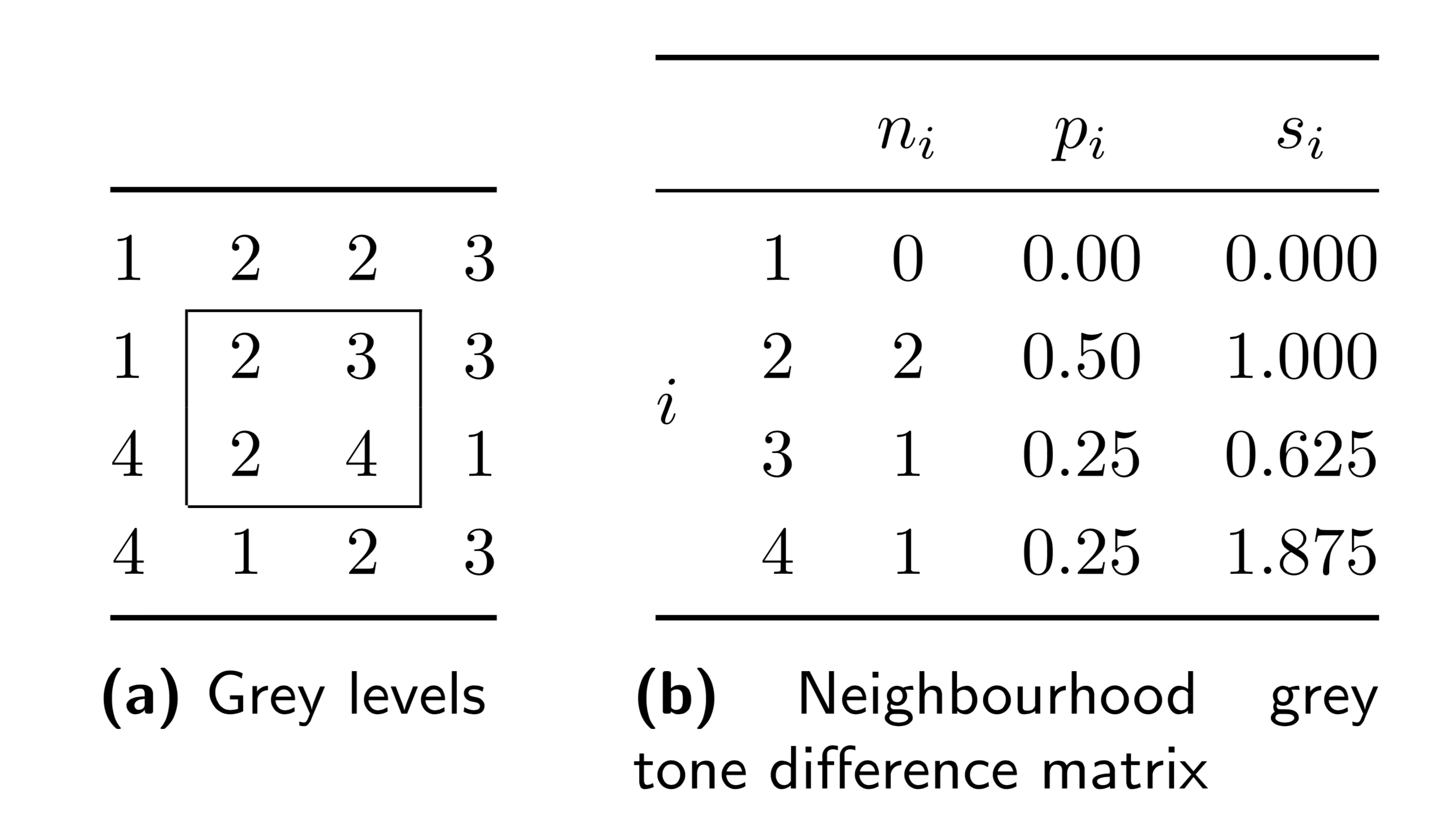
Fig. 18 Original image with grey levels (a) and corresponding neighbourhood grey tone difference matrix (NGTDM) (b). The \(N_{v,c}\) pixels with valid neighbours at distance 1 are located within the rectangle in (a). The grey level voxel count \(n_i\), the grey level probability \(p_i=n_i/N_{v,c}\), and the neighbourhood grey level difference \(s_i\) for pixels with grey level \(i\) are included in the NGTDM. Note that our actual definition deviates from the original definition of [Amadasun1989], which is used here. In our definition complete neighbourhood are no longer required. In our definition the NGTDM would be calculated on the entire pixel area, and not solely on those pixels within the rectangle of panel (a).

Aggregating features

Three methods can be used to aggregate NGTDMs and arrive at a single feature value. A schematic example was previously shown in Fig. 16. A feature may be aggregated as follows:

1. Features are computed from 2D matrices and averaged over slices (8QNN).
2. The feature is computed from a single matrix after merging all 2D matrices (62GR).
3. The feature is computed from a 3D matrix (KOBO).

Method 2 involves merging NGTDMs by summing the neighbourhood grey tone difference \(s_i\) and the number of voxels with a valid neighbourhood \(n_i\) and grey level \(i\) for NGTDMs of the different slices. Note that when NGTDMs are merged, \(N_{v,c}\) and \(p_i\) should be updated based on the merged NGTDM. Feature values may dependent strongly on the aggregation method.

Distances and distance weighting

The default neighbourhood is defined using the Chebyshev norm. Manhattan or Euclidean norms may be used as well. This requires a more general definition for the average grey level \(\overline{X}_k\):

\[\overline{X}_k =\frac{1}{W_k}\sum_{m_z{=}-\delta}^\delta \sum_{m_y{=}-\delta}^\delta \sum_{m_x{=}-\delta}^\delta X_{d}(\mathbf{k}+\mathbf{m}) \big[\|\mathbf{m}\|\leq\delta \text{ and } \mathbf{m\neq\mathbf{0}} \text{ and } \mathbf{k}+\mathbf{m} \text{ in ROI}\big]\]

The neighbourhood size \(W_k\) is:

\[W_k = \sum_{m_z{=}-\delta}^\delta \sum_{m_y{=}-\delta}^\delta \sum_{m_x{=}-\delta}^\delta \big[\|\mathbf{m}\|\leq\delta \text{ and } \mathbf{m\neq\mathbf{0}} \text{ and } \mathbf{k}+\mathbf{m} \text{ in ROI}\big]\]

As before, \(\big[\ldots\big]\) is an Iverson bracket.

Distance weighting for NGTDM is relatively straightforward. Let \(w\) be a weight dependent on \(\mathbf{m}\), e.g. \(w=\|\mathbf{m}\|^{-1}\) or \(w=\exp(-\|\mathbf{m}\|^2)\). The average grey level is then:

\[\overline{X}_k =\frac{1}{W_k}\sum_{m_z{=}-\delta}^\delta \sum_{m_y{=}-\delta}^\delta \sum_{m_x{=}-\delta}^\delta w(\mathbf{m}) X_{d}(\mathbf{k}+\mathbf{m}) \big[\|\mathbf{m}\|\leq\delta \text{ and } \mathbf{m\neq\mathbf{0}} \text{ and } \mathbf{k}+\mathbf{m} \text{ in ROI}\big]\]

The neighbourhood size \(W_k\) becomes a general weight:

\[W_k = \sum_{m_z{=}-\delta}^\delta \sum_{m_y{=}-\delta}^\delta \sum_{m_x{=}-\delta}^\delta w(\mathbf{m}) \big[\|\mathbf{m}\|\leq\delta \text{ and } \mathbf{m\neq\mathbf{0}} \text{ and } \mathbf{k}+\mathbf{m} \text{ in ROI}\big]\]

Employing different distance norms and distance weighting is considered non-standard use, and we caution against them due to potential reproducibility issues.

Coarseness

QCDE

Grey level differences in coarse textures are generally small due to large-scale patterns. Summing differences gives an indication of the level of the spatial rate of change in intensity [Amadasun1989]. Coarseness is defined as:

\[F_{\mathit{ngt.coarseness}}=\frac{1}{\sum_{i=1}^{N_g} p_i\,s_i }\]

Because \(\sum_{i=1}^{N_g} p_i\,s_i\) potentially evaluates to 0, the maximum coarseness value is set to an arbitrary number of \(10^6\). Amadasun and King originally circumvented this issue by adding a unspecified small number \(\epsilon\) to the denominator, but an explicit, though arbitrary, maximum value should allow for more consistency.

data	aggr. method	value	tol.	consensus
dig. phantom	2D	0.121	—	strong
dig. phantom	2.5D	0.0285	—	strong
dig. phantom	3D	0.0296	—	very strong
config. A	2D	0.00629	0.00046	strong
config. A	2.5D	\(9.06 \times 10^{-5}\)	\(3.3 \times 10^{-6}\)	strong
config. B	2D	0.0168	0.0005	strong
config. B	2.5D	0.000314	\(4 \times 10^{-6}\)	strong
config. C	3D	0.000216	\(4 \times 10^{-6}\)	strong
config. D	3D	0.000208	\(4 \times 10^{-6}\)	very strong
config. E	3D	0.000188	\(4 \times 10^{-6}\)	strong

Contrast

65HE

Contrast depends on the dynamic range of the grey levels as well as the spatial frequency of intensity changes [Amadasun1989]. Thus, contrast is defined as:

\[F_{\mathit{ngt.contrast}}=\left(\frac{1}{N_{g,p}\left(N_{g,p}-1\right)} \sum_{i_{1}=1}^{N_g} \sum_{i_{2}=1}^{N_g} p_{i_{1}} p_{i_{2}}\,(i_{1}-i_{2})^2 \right) \left( \frac{1}{N_{v,c}}\sum_{i=1}^{N_g} s_i \right)\]

Grey level probabilities \(p_{i_{1}}\) and \(p_{i_{2}}\) are copies of \(p_i\) with different iterators, i.e. \(p_{i_{1}}=p_{i_{2}}\) for \(i_{1}=i_{2}\). The first term considers the grey level dynamic range, whereas the second term is a measure for intensity changes within the volume. If \(N_{g,p}=1\), \(F_{\mathit{ngt.contrast}}=0\).

data	aggr. method	value	tol.	consensus
dig. phantom	2D	0.925	—	strong
dig. phantom	2.5D	0.601	—	strong
dig. phantom	3D	0.584	—	very strong
config. A	2D	0.107	0.002	strong
config. A	2.5D	0.0345	0.0009	strong
config. B	2D	0.181	0.001	strong
config. B	2.5D	0.0506	0.0005	strong
config. C	3D	0.0873	0.0019	strong
config. D	3D	0.046	0.0005	strong
config. E	3D	0.0752	0.0019	strong

Busyness

NQ30

Textures with large changes in grey levels between neighbouring voxels are said to be busy [Amadasun1989]. Busyness was defined as:

\[F_{\mathit{ngt.busyness}}=\frac{\sum_{i=1}^{N_g}p_i\,s_i}{\sum_{i_{1}=1}^{N_g}\sum_{i_2=1}^{N_g} i_{1} \, p_{i_{1}}- i_{2} \, p_{i_{2}}},\qquad \text{$p_{i_{1}}\neq 0$ \text{and} $p_{i_{2}}\neq 0$}\]

As before, \(p_{i_{1}}=p_{i_{2}}\) for \(i_{1}=i_{2}\). The original definition was erroneously formulated as the denominator will always evaluate to 0. Therefore we use a slightly different definition [Hatt2016]:

\[F_{\mathit{ngt.busyness}}=\frac{\sum_{i=1}^{N_g}p_i\,s_i}{\sum_{i_{1}=1}^{N_g}\sum_{i_{2}=1}^{N_g} \left| i_{1} \, p_{i_{1}}-i_{2} \, p_{i_{2}}\right|},\qquad \text{$p_{i_{1}}\neq 0$ \text{and} $p_{i_{2}}\neq 0$}\]

If \(N_{g,p}=1\), \(F_{\mathit{ngt.busyness}}=0\).

data	aggr. method	value	tol.	consensus
dig. phantom	2D	2.99	—	strong
dig. phantom	2.5D	6.8	—	strong
dig. phantom	3D	6.54	—	very strong
config. A	2D	0.489	0.001	strong
config. A	2.5D	8.84	0.01	strong
config. B	2D	0.2	0.005	strong
config. B	2.5D	3.45	0.07	strong
config. C	3D	1.39	0.01	strong
config. D	3D	5.14	0.14	very strong
config. E	3D	4.65	0.1	strong

Complexity

HDEZ

Complex textures are non-uniform and rapid changes in grey levels are common [Amadasun1989]. Texture complexity is defined as:

\[F_{\mathit{ntg.complexity}}=\frac{1}{N_{v,c}}\sum_{i_{1}=1}^{N_g}\sum_{i_{2}=1}^{N_g} \left| i_{1} - i_{2}\right| \frac{p_{i_{1}}\, s_{i_{1}} + p_{i_{2}}\,s_{i_{2}}}{p_{i_{1}} + p_{i_{2}}}, \qquad \text{$p_{i_{1}}\neq 0$ \text{and} $p_{i_{2}}\neq 0$}\]

As before, \(p_{i_{1}}=p_{i_{2}}\) for \(i_{1}=i_{2}\), and likewise \(s_{i_{1}}=s_{i_{2}}\) for \(i_{1}=i_{2}\).

data	aggr. method	value	tol.	consensus
dig. phantom	2D	10.4	—	strong
dig. phantom	2.5D	14.1	—	strong
dig. phantom	3D	13.5	—	very strong
config. A	2D	438	9	strong
config. A	2.5D	580	19	strong
config. B	2D	391	7	strong
config. B	2.5D	496	5	strong
config. C	3D	\(1.81 \times 10^{3}\)	60	strong
config. D	3D	400	5	strong
config. E	3D	574	1	strong

Strength

1X9X

[Amadasun1989] defined texture strength as:

\[F_{\mathit{ngt.strength}}=\frac{\sum_{i_{1}=1}^{N_g}\sum_{i_{2}=1}^{N_g}\left( p_{i_{1}} + p_{i_{2}} \right) \left( i_{1} - i_{2}\right)^2 }{\sum_{i=1}^{N_g}s_i},\qquad \text{$p_{i_{1}}\neq 0$ \text{and} $p_{i_{2}}\neq 0$}\]

As before, \(p_{i_{1}}=p_{i_{2}}\) for \(i_{1}=i_{2}\). If \(\sum_{i=1}^{N_g}s_i=0\), \(F_{\mathit{ngt.strength}}=0\).

data	aggr. method	value	tol.	consensus
dig. phantom	2D	2.88	—	strong
dig. phantom	2.5D	0.741	—	strong
dig. phantom	3D	0.763	—	very strong
config. A	2D	3.33	0.08	strong
config. A	2.5D	0.0904	0.0027	strong
config. B	2D	6.02	0.23	strong
config. B	2.5D	0.199	0.009	strong
config. C	3D	0.651	0.015	strong
config. D	3D	0.162	0.008	very strong
config. E	3D	0.167	0.006	strong

Neighbouring grey level dependence based features

REK0

[Sun1983] defined the neighbouring grey level dependence matrix (NGLDM) as an alternative to the grey level co-occurrence matrix. The NGLDM aims to capture the coarseness of the overall texture and is rotationally invariant.

NGLDM also involves the concept of a neighbourhood around a central voxel. All voxels within Chebyshev distance \(\delta\) are considered to belong to the neighbourhood of the center voxel. The discretised grey levels of the center voxel \(k\) at position \(\mathbf{k}\) and a neighbouring voxel \(m\) at \(\mathbf{k}+\mathbf{m}\) are said to be dependent if \(|X_d(\mathbf{k}) - X_d(\mathbf{k}+\mathbf{m}) | \leq \alpha\), with \(\alpha\) being a non-negative integer coarseness parameter. The number of grey level dependent voxels \(j\) within the neighbourhood is then counted as:

\[j_k = 1+\sum_{m_z{=}-\delta}^\delta \sum_{m_y{=}-\delta}^\delta \sum_{m_x{=}-\delta}^\delta \big[|X_{d}(\mathbf{k})-X_{d}(\mathbf{k}+\mathbf{m})| \leq \alpha \text{ and } \mathbf{m}\neq\mathbf{0}\big]\]

Here, \(\big[\ldots\big]\) is an Iverson bracket, which is \(1\) if the aforementioned condition is fulfilled, and \(0\) otherwise. Note that the minimum dependence \(j_k=1\) and not \(j_k=0\). This is done because some feature definitions require a minimum dependence of 1 or are undefined otherwise. One may therefore also simplify the expression for \(j_k\) by including the center voxel:

\[j_k = \sum_{m_z{=}-\delta}^\delta \sum_{m_y{=}-\delta}^\delta \sum_{m_x{=}-\delta}^\delta \big[|X_{d}(\mathbf{k})-X_{d}(\mathbf{k}+\mathbf{m})| \leq \alpha\big]\]

Dependence \(j_k\) is iteratively determined for each voxel \(k\) in the ROI intensity mask. \(\mathbf{M}\) is then the \(N_g \times N_n\) neighbouring grey level dependence matrix, where \(N_g\) is the number of discretised grey levels present in the ROI intensity mask and \(N_n=\text{max}(j_k)\) the maximum grey level dependence count found. Element \(s_{ij}\) of \(\mathbf{M}\) is then the number of neighbourhoods with a center voxel with discretised grey level \(i\) and a neighbouring voxel dependence \(j\). Furthermore, let \(N_v\) be the number of voxels in the ROI intensity mask, and \(N_s = \sum_{i=1}^{N_g}\sum_{j=1}^{N_n} s_{ij}\) the number of neighbourhoods. Marginal sums can likewise be defined. Let \(s_{i.}=\sum_{j=1}^{N_n}\) be the number of neighbourhoods with discretised grey level \(i\), and let \(s_{j.}=\sum_{i=1}^{N_g}s_{ij}\) be the number of neighbourhoods with dependence \(j\), regardless of grey level. A two dimensional example is shown in Fig. 19.

The definition we actually use deviates from the original by [Sun1983]. Because regions of interest are rarely cuboid, omission of neighbourhoods which contain voxels outside the ROI mask may lead to inconsistent results, especially for larger distance \(\delta\). Hence the neighbourhoods of all voxels in the within the ROI intensity mask are considered, and consequently \(N_v=N_s\). Neighbourhood voxels located outside the ROI do not add to dependence \(j\):

\[j_k = \sum_{m_z{=}-\delta}^\delta \sum_{m_y{=}-\delta}^\delta \sum_{m_x{=}-\delta}^\delta \big[|X_{d}(\mathbf{k})-X_{d}(\mathbf{k}+\mathbf{m})| \leq \alpha \text{ and } \mathbf{k}+\mathbf{m} \text{ in ROI}\big]\]

Note that while \(\alpha=0\) is a typical choice for the coarseness parameter, different \(\alpha\) are possible. Likewise, a typical choice for neighbourhood radius \(\delta\) is Chebyshev distance \(\delta=1\) but larger values are possible as well.

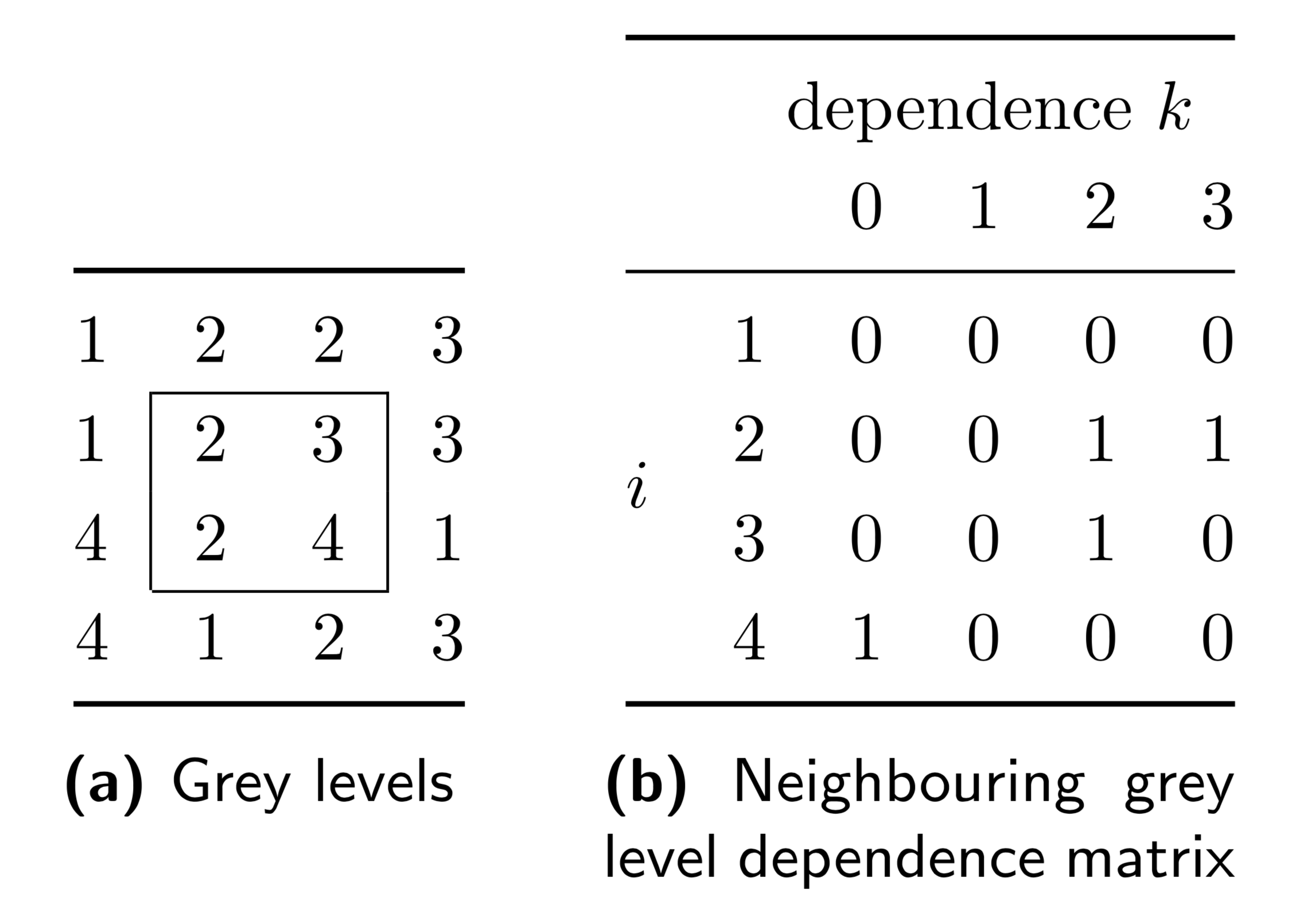
Fig. 19 Original image with grey levels and pixels with a complete neighbourhood within the square (a); corresponding neighbouring grey level dependence matrix for distance \(d = \sqrt{2}\) and coarseness parameter \(a = 0\) (b). Element \(s_{i,j}\) of the NGLDM indicates the number of neighbourhoods with a center pixel with grey level i and neighbouring grey level dependence k within the image. Note that in our definition a complete neighbourhood is no longer required. Thus every voxel is considered as a center voxel with a neighbourhood, instead of being constrained to the voxels within the square in panel (a).

Aggregating features

Three methods can be used to aggregate NGLDMs and arrive at a single feature value. A schematic example was previously shown in Fig. 16. A feature may be aggregated as follows:

1. Features are computed from 2D matrices and averaged over slices (8QNN).
2. The feature is computed from a single matrix after merging all 2D matrices (62GR).
3. The feature is computed from a 3D matrix (KOBO).

Method 2 involves merging NGLDMs by summing the dependence count \(s_{ij}\) by element over the NGLDM of the different slices. Note that when NGLDMs are merged, \(N_v\) and \(N_s\) should likewise be summed to retain consistency. Feature values may dependent strongly on the aggregation method.

Distances and distance weighting

Default neighbourhoods are constructed using the Chebyshev norm, but other norms can be used as well. For this purpose it is useful to generalise the dependence count equation to:

\[j_k = \sum_{m_z{=}-\delta}^\delta \sum_{m_y{=}-\delta}^\delta \sum_{m_x{=}-\delta}^\delta \big[\|\mathbf{m}\|\leq\delta \text{ and } |X_{d}(\mathbf{k})-X_{d}(\mathbf{k}+\mathbf{m})| \leq \alpha \text{ and } \mathbf{k}+\mathbf{m} \text{ in ROI}\big]\]

with \(\mathbf{m}\) the vector between voxels \(k\) and \(m\) and \(\|\mathbf{m}\|\) its length according to the particular norm.

In addition, dependence may be weighted by distance. Let \(w\) be a weight dependent on \(\mathbf{m}\), e.g. \(w=\|\mathbf{m}\|^{-1}\) or \(w=\exp(-\|\mathbf{m}\|^2)\). The dependence of voxel \(k\) is then:

\[j_k = \sum_{m_z{=}-\delta}^\delta \sum_{m_y{=}-\delta}^\delta \sum_{m_x{=}-\delta}^\delta w(\mathbf{m}) \big[\|\mathbf{m}\|\leq\delta \text{ and } |X_{d}(\mathbf{k})-X_{d}(\mathbf{k}+\mathbf{m})| \leq \alpha \text{ and } \mathbf{k}+\mathbf{m} \text{ in ROI}\big]\]

Employing different distance norms and distance weighting is considered non-standard use, and we caution against them due to potential reproducibility issues.

Note on feature references

The NGLDM is structured similarly to the GLRLM, GLSZM and GLDZM. NGLDM feature definitions are therefore based on the definitions of GLRLM features, and references may be found in Grey level run length based features, except for the features originally defined by [Sun1983].

Low dependence emphasis

SODN

This feature emphasises low neighbouring grey level dependence counts. [Sun1983] refer to this feature as small number emphasis. It is defined as:

\[F_{\mathit{ngl.lde}} = \frac{1}{N_s} \sum_{j=1}^{N_n} \frac{s_{.j}}{j^2}\]

data	aggr. method	value	tol.	consensus
dig. phantom	2D	0.158	—	strong
dig. phantom	2.5D	0.159	—	strong
dig. phantom	3D	0.045	—	very strong
config. A	2D	0.281	0.003	strong
config. A	2.5D	0.243	0.004	strong
config. B	2D	0.31	0.001	strong
config. B	2.5D	0.254	0.002	strong
config. C	3D	0.137	0.003	strong
config. D	3D	0.0912	0.0007	strong
config. E	3D	0.118	0.001	strong

High dependence emphasis

IMOQ

This feature emphasises high neighbouring grey level dependence counts. [Sun1983] refer to this feature as large number emphasis. It is defined as:

\[F_{\mathit{ngl.hde}} = \frac{1}{N_s} \sum_{j=1}^{N_n} j^2 s_{.j}\]

data	aggr. method	value	tol.	consensus
dig. phantom	2D	19.2	—	strong
dig. phantom	2.5D	18.8	—	strong
dig. phantom	3D	109	—	very strong
config. A	2D	14.8	0.1	strong
config. A	2.5D	16.1	0.2	strong
config. B	2D	17.3	0.2	strong
config. B	2.5D	19.6	0.2	strong
config. C	3D	126	2	strong
config. D	3D	223	5	strong
config. E	3D	134	3	strong

Low grey level count emphasis

TL9H

This feature is a grey level analogue to low dependence emphasis. Instead of low neighbouring grey level dependence counts, low grey levels are emphasised. The feature is defined as:

\[F_{\mathit{ngl.lgce}}=\frac{1}{N_s} \sum_{i=1}^{N_g} \frac{s_{i.}}{i^2}\]

data	aggr. method	value	tol.	consensus
dig. phantom	2D	0.702	—	strong
dig. phantom	2.5D	0.693	—	strong
dig. phantom	3D	0.693	—	very strong
config. A	2D	0.0233	0.0003	strong
config. A	2.5D	0.0115	0.0003	strong
config. B	2D	0.0286	0.0004	strong
config. B	2.5D	0.0139	0.0005	strong
config. C	3D	0.0013	\(4 \times 10^{-5}\)	strong
config. D	3D	0.0168	0.0009	strong
config. E	3D	0.0154	0.0007	strong

High grey level count emphasis

OAE7

The high grey level count emphasis feature is a grey level analogue to high dependence emphasis. The feature emphasises high grey levels, and is defined as:

\[F_{\mathit{ngl.hgce}}=\frac{1}{N_s} \sum_{i=1}^{N_g} i^2 s_{i.}\]

data	aggr. method	value	tol.	consensus
dig. phantom	2D	7.49	—	strong
dig. phantom	2.5D	7.66	—	strong
dig. phantom	3D	7.66	—	very strong
config. A	2D	446	2	strong
config. A	2.5D	466	2	strong
config. B	2D	359	10	strong
config. B	2.5D	375	11	strong
config. C	3D	\(1.57 \times 10^{3}\)	10	strong
config. D	3D	364	16	strong
config. E	3D	502	8	strong

Low dependence low grey level emphasis

EQ3F

This feature emphasises neighbouring grey level dependence counts in the upper left quadrant of the NGLDM, where low dependence counts and low grey levels are located. It is defined as:

\[F_{\mathit{ngl.ldlge}}=\frac{1}{N_s} \sum_{i=1}^{N_g} \sum_{j=1}^{N_n} \frac{s_{ij}}{i^2 j^2}\]

data	aggr. method	value	tol.	consensus
dig. phantom	2D	0.0473	—	strong
dig. phantom	2.5D	0.0477	—	strong
dig. phantom	3D	0.00963	—	very strong
config. A	2D	0.0137	0.0002	strong
config. A	2.5D	0.00664	0.0002	strong
config. B	2D	0.0203	0.0003	strong
config. B	2.5D	0.00929	0.00026	strong
config. C	3D	0.000306	\(1.2 \times 10^{-5}\)	strong
config. D	3D	0.00357	\(4 \times 10^{-5}\)	strong
config. E	3D	0.00388	\(4 \times 10^{-5}\)	strong

Low dependence high grey level emphasis

JA6D

This feature emphasises neighbouring grey level dependence counts in the lower left quadrant of the NGLDM, where low dependence counts and high grey levels are located. The feature is defined as:

\[F_{\mathit{ngl.ldhge}}=\frac{1}{N_s} \sum_{i=1}^{N_g} \sum_{j=1}^{N_n} \frac{i^2 s_{ij}}{j^2}\]

data	aggr. method	value	tol.	consensus
dig. phantom	2D	3.06	—	strong
dig. phantom	2.5D	3.07	—	strong
dig. phantom	3D	0.736	—	very strong
config. A	2D	94.2	0.4	strong
config. A	2.5D	91.9	0.5	strong
config. B	2D	78.9	2.2	strong
config. B	2.5D	73.4	2.1	strong
config. C	3D	141	2	strong
config. D	3D	18.9	1.1	strong
config. E	3D	36.7	0.5	strong

High dependence low grey level emphasis

NBZI

This feature emphasises neighbouring grey level dependence counts in the upper right quadrant of the NGLDM, where high dependence counts and low grey levels are located. The feature is defined as:

\[F_{\mathit{ngl.hdlge}}=\frac{1}{N_s} \sum_{i=1}^{N_g} \sum_{j=1}^{N_n} \frac{j^2 s_{ij}}{i^2}\]

data	aggr. method	value	tol.	consensus
dig. phantom	2D	17.6	—	strong
dig. phantom	2.5D	17.2	—	strong
dig. phantom	3D	102	—	very strong
config. A	2D	0.116	0.001	strong
config. A	2.5D	0.0674	0.0004	strong
config. B	2D	0.108	0.003	strong
config. B	2.5D	0.077	0.0019	strong
config. C	3D	0.0828	0.0003	strong
config. D	3D	0.798	0.072	strong
config. E	3D	0.457	0.031	strong

High dependence high grey level emphasis

9QMG

The high dependence high grey level emphasis feature emphasises neighbouring grey level dependence counts in the lower right quadrant of the NGLDM, where high dependence counts and high grey levels are located. The feature is defined as:

\[F_{\mathit{ngl.hdhge}}=\frac{1}{N_s} \sum_{i=1}^{N_g} \sum_{j=1}^{N_n} i^2 j^2 s_{ij}\]

data	aggr. method	value	tol.	consensus
dig. phantom	2D	49.5	—	strong
dig. phantom	2.5D	50.8	—	strong
dig. phantom	3D	235	—	very strong
config. A	2D	\(7.54 \times 10^{3}\)	60	strong
config. A	2.5D	\(8.1 \times 10^{3}\)	60	strong
config. B	2D	\(7.21 \times 10^{3}\)	130	strong
config. B	2.5D	\(7.97 \times 10^{3}\)	150	strong
config. C	3D	\(2.27 \times 10^{5}\)	\(3 \times 10^{3}\)	strong
config. D	3D	\(9.28 \times 10^{4}\)	\(1.3 \times 10^{3}\)	strong
config. E	3D	\(7.6 \times 10^{4}\)	600	strong

Grey level non-uniformity

FP8K

Grey level non-uniformity assesses the distribution of neighbouring grey level dependence counts over the grey values. The feature value is low when dependence counts are equally distributed along grey levels. The feature is defined as:

\[F_{\mathit{ngl.glnu}}= \frac{1}{N_s} \sum_{i=1}^{N_g} s_{i.}^2\]

data	aggr. method	value	tol.	consensus
dig. phantom	2D	10.2	—	strong
dig. phantom	2.5D	37.9	—	strong
dig. phantom	3D	37.9	—	very strong
config. A	2D	757	1	strong
config. A	2.5D	\(1.72 \times 10^{4}\)	100	strong
config. B	2D	216	3	strong
config. B	2.5D	\(4.76 \times 10^{3}\)	50	strong
config. C	3D	\(6.42 \times 10^{3}\)	10	strong
config. D	3D	\(1.02 \times 10^{4}\)	300	strong
config. E	3D	\(8.17 \times 10^{3}\)	130	strong

Normalised grey level non-uniformity

5SPA

This is a normalised version of the grey level non-uniformity feature. It is defined as:

\[F_{\mathit{ngl.glnu.norm}}= \frac{1}{N_s^2} \sum_{i=1}^{N_g} s_{i.}^2\]

The normalised grey level non-uniformity computed from a single 3D NGLDM matrix is equivalent to the intensity histogram uniformity feature [VanGriethuysen2017].

data	aggr. method	value	tol.	consensus
dig. phantom	2D	0.562	—	strong
dig. phantom	2.5D	0.512	—	strong
dig. phantom	3D	0.512	—	very strong
config. A	2D	0.151	0.003	strong
config. A	2.5D	0.15	0.002	strong
config. B	2D	0.184	0.001	strong
config. B	2.5D	0.174	0.001	strong
config. C	3D	0.14	0.003	strong
config. D	3D	0.229	0.003	strong
config. E	3D	0.184	0.001	strong

Dependence count non-uniformity

Z87G

This features assesses the distribution of neighbouring grey level dependence counts over the different dependence counts. The feature value is low when dependence counts are equally distributed. [Sun1983] refer to this feature as number non-uniformity. It is defined as:

\[F_{\mathit{ngl.dcnu}}= \frac{1}{N_s} \sum_{j=1}^{N_n} s_{.j}^2\]

data	aggr. method	value	tol.	consensus
dig. phantom	2D	3.96	—	strong
dig. phantom	2.5D	12.4	—	strong
dig. phantom	3D	4.86	—	very strong
config. A	2D	709	2	strong
config. A	2.5D	\(1.75 \times 10^{4}\)	100	strong
config. B	2D	157	1	strong
config. B	2.5D	\(3.71 \times 10^{3}\)	30	strong
config. C	3D	\(2.45 \times 10^{3}\)	60	strong
config. D	3D	\(1.84 \times 10^{3}\)	30	strong
config. E	3D	\(2.25 \times 10^{3}\)	30	strong

Normalised dependence count non-uniformity

OKJI

This is a normalised version of the dependence count non-uniformity feature. It is defined as:

\[F_{\mathit{ngl.dcnu.norm}}= \frac{1}{N_s^2} \sum_{i=1}^{N_n} s_{.j}^2\]

data	aggr. method	value	tol.	consensus
dig. phantom	2D	0.212	—	strong
dig. phantom	2.5D	0.167	—	strong
dig. phantom	3D	0.0657	—	very strong
config. A	2D	0.175	0.001	strong
config. A	2.5D	0.153	0.001	strong
config. B	2D	0.179	0.001	strong
config. B	2.5D	0.136	0.001	strong
config. C	3D	0.0532	0.0005	strong
config. D	3D	0.0413	0.0003	strong
config. E	3D	0.0505	0.0003	strong

Dependence count percentage

6XV8

This feature measures the fraction of the number of realised neighbourhoods and the maximum number of potential neighbourhoods. Dependence count percentage may be completely omitted as it evaluates to \(1\) when complete neighbourhoods are not required, as is the case under our definition. It is defined as:

\[F_{\mathit{ngl.dc.perc}}=\frac{N_s}{N_v}\]

data	aggr. method	value	tol.	consensus
dig. phantom	2D	1	—	strong
dig. phantom	2.5D	1	—	moderate
dig. phantom	3D	1	—	strong
config. A	2D	1	—	moderate
config. A	2.5D	1	—	moderate
config. B	2D	1	—	moderate
config. B	2.5D	1	—	moderate
config. C	3D	1	—	strong
config. D	3D	1	—	strong
config. E	3D	1	—	moderate

Grey level variance

1PFV

This feature estimates the variance in dependence counts over the grey levels. Let \(p_{ij} = s_{ij}/N_s\) be the joint probability estimate for finding discretised grey level \(i\) with dependence \(j\). The feature is then defined as:

\[F_{\mathit{ngl.gl.var}}= \sum_{i=1}^{N_g} \sum_{j=1}^{N_n} (i-\mu)^2 p_{ij}\]

Here, \(\mu = \sum_{i=1}^{N_g} \sum_{j=1}^{N_n} i\,p_{ij}\).

data	aggr. method	value	tol.	consensus
dig. phantom	2D	2.7	—	strong
dig. phantom	2.5D	3.05	—	strong
dig. phantom	3D	3.05	—	very strong
config. A	2D	31.1	0.5	strong
config. A	2.5D	22.8	0.6	strong
config. B	2D	25.3	0.4	strong
config. B	2.5D	18.7	0.2	strong
config. C	3D	81.1	2.1	strong
config. D	3D	21.7	0.4	strong
config. E	3D	30.4	0.8	strong

}

Dependence count variance

DNX2

This feature estimates the variance in dependence counts over the different possible dependence counts. As before let \(p_{ij} = s_{ij}/N_s\). The feature is defined as:

\[F_{\mathit{ngl.dc.var}}= \sum_{i=1}^{N_g} \sum_{j=1}^{N_n} (j-\mu)^2 p_{ij}\]

Mean dependence count is defined as \(\mu = \sum_{i=1}^{N_g} \sum_{j=1}^{N_n} j\,p_{ij}\).

data	aggr. method	value	tol.	consensus
dig. phantom	2D	2.73	—	strong
dig. phantom	2.5D	3.27	—	strong
dig. phantom	3D	22.1	—	very strong
config. A	2D	3.12	0.02	strong
config. A	2.5D	3.37	0.01	strong
config. B	2D	4.02	0.05	strong
config. B	2.5D	4.63	0.06	strong
config. C	3D	39.2	0.1	strong
config. D	3D	63.9	1.3	strong
config. E	3D	39.4	1	strong

Dependence count entropy

FCBV

This feature is referred to as entropy by [Sun1983]. Let \(p_{ij} = s_{ij}/N_s\). Dependence count entropy is then defined as:

\[F_{\mathit{ngl.dc.entr}} = - \sum_{i=1}^{N_g} \sum_{j=1}^{N_n} p_{ij} \log_2 p_{ij}\]

This definition remedies an error in the definition of [Sun1983], where the term within the logarithm is dependence count \(s_{ij}\) instead of count probability \(p_{ij}\).

data	aggr. method	value	tol.	consensus
dig. phantom	2D	2.71	—	strong
dig. phantom	2.5D	3.36	—	strong
dig. phantom	3D	4.4	—	very strong
config. A	2D	5.76	0.02	strong
config. A	2.5D	5.93	0.02	strong
config. B	2D	5.38	0.01	strong
config. B	2.5D	5.78	0.01	strong
config. C	3D	7.54	0.03	strong
config. D	3D	6.98	0.01	strong
config. E	3D	7.06	0.02	strong

Dependence count energy

CAS9

This feature is called second moment by [Sun1983]. Let \(p_{ij} = s_{ij}/N_s\). Then dependence count energy is defined as:

\[F_{\mathit{ngl.dc.energy}} = \sum_{i=1}^{N_g} \sum_{j=1}^{N_n} p_{ij}^2\]

This definition also remedies an error in the original definition, where squared dependence count \(s_{ij}^2\) is divided by \(N_s\) only, thus leaving a major volume dependency. In the definition given here, \(s_{ij}^2\) is normalised by \(N_s^2\) through the use of count probability \(p_{ij}\).

data	aggr. method	value	tol.	consensus
dig. phantom	2D	0.17	—	strong
dig. phantom	2.5D	0.122	—	strong
dig. phantom	3D	0.0533	—	very strong
config. A	2D	0.0268	0.0004	strong
config. A	2.5D	0.0245	0.0003	moderate
config. B	2D	0.0321	0.0002	strong
config. B	2.5D	0.0253	0.0001	moderate
config. C	3D	0.00789	0.00011	strong
config. D	3D	0.0113	0.0002	strong
config. E	3D	0.0106	0.0001	strong