Image processing
Image processing is the sequence of operations required to derive image biomarkers (features) from acquired images. In the context of this work an image is defined as a three-dimensional (3D) stack of two-dimensional (2D) digital image slices. Image slices are stacked along the \(z\)-axis. This stack is furthermore assumed to possess the same coordinate system, i.e. image slices are not rotated or translated (in the \(xy\)-plane) with regards to each other. Moreover, digital images typically possess a finite resolution. Intensities in an image are thus located at regular intervals, or spacing. In 2D such regular positions are called pixels, whereas in 3D the term voxels is used. Pixels and voxels are thus represented as the intersections on a regularly spaced grid. Alternatively, pixels and voxels may be represented as rectangles and rectangular cuboids. The centers of the pixels and voxels then coincide with the intersections of the regularly spaced grid. Both representations are used in the document.
Pixels and voxels contain an intensity value for each channel of the image. The number of channels depends on the imaging modality. Most medical imaging generates single-channel images, whereas the number of channels in microscopy may be greater, e.g. due to different stainings. In such multi-channel cases, features may be extracted for each separate channel, a subset of channels, or alternatively, channels may be combined and converted to a single-channel representation. In the remainder of the document we consider an image as if it only possesses a single channel.
The intensity of a pixel or voxel is also called a grey level or grey tone, particularly in single-channel images. Though practically there is no difference, the terms grey level or grey tone are more commonly used to refer to discrete intensities, including discretised intensities.
Image processing may be conducted using a wide variety of schemes. We therefore designed a general image processing scheme for image feature calculation based on schemes used within scientific literature [Hatt2016]. The image processing scheme is shown in Fig. 1. The processing steps referenced in the figure are described in detail within this chapter.
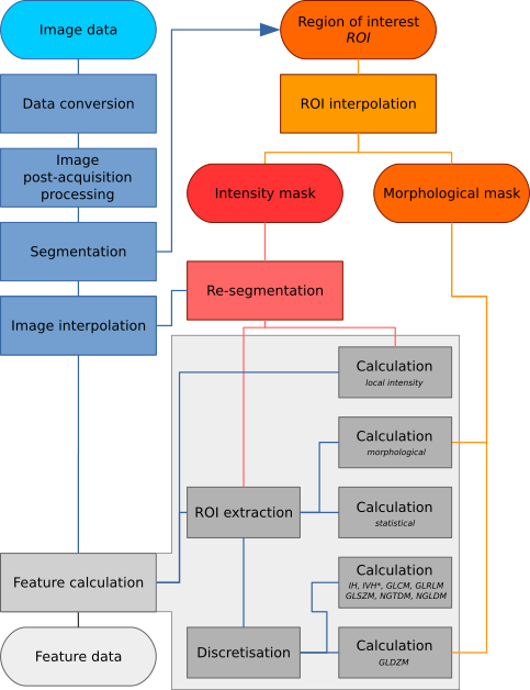
Fig. 1 Image processing scheme for image feature calculation. Depending on the specific imaging modality and purpose, some steps may be omitted. The region of interest (ROI) is explicitly split into two masks, namely an intensity and morphological mask, after interpolation to the same grid as the interpolated image. Feature calculation is expanded to show the different feature families with specific pre-processing. IH: intensity histogram; IVH: intensity-volume histogram; GLCM: grey level cooccurrence matrix; GLRLM: grey level run length matrix; GLSZM: grey level size zone matrix; NGTDM: neighbourhood grey tone difference matrix; NGLDM: Neighbouring grey level dependence matrix; GLDZM: grey level distance zone matrix; *Discretisation of IVH differs from IH and texture features (see Intensity-volume histogram features).
Data conversion
23XZ
Some imaging modalities require conversion of raw image data into a more meaningful presentation, e.g. standardised uptake values (SUV) [Boellaard2015]. This is performed during the data conversion step. Assessment of data conversion methods falls outside the scope of the current work.
Image post-acquisition processing
PCDE
Images are post-processed to enhance image quality. For instance, magnetic resonance imaging (MRI) contains both Gaussian and Rician noise [Gudbjartsson1995] and may benefit from denoising. As another example, intensities measured using MR may be non-uniform across an image and could require correction [Sled1998][Vovk2007][Balafar2010]. FDG-PET-based may furthermore be corrected for partial volume effects [Soret2007][Boussion2009] and noise [LePogam2013][ElNaqa2017]. In CT imaging, metal objects, e.g. pacemakers and tooth implants, introduce artifacts and may require artifinterpact suppression [Gjesteby2016]. Microscopy images generally benefit from field-of-view illumination correction as illumination is usually inhomogeneous due to the light-source or the optical path [Caicedo2017][Smith2015].
Evaluation and standardisation of various image post-acquisition processing methods falls outside the scope of the current work. Note that vendors may provide or implement software to perform noise reduction and other post-processing during image reconstruction. In such cases, additional post-acquisition processing may not be required.
Segmentation
OQYT
High-throughput image analysis, within the feature-based paradigm, relies on the definition of regions of interest (ROI). ROIs are used to define the region in which features are calculated. What constitutes an ROI depends on the imaging and the study objective. For example, in 3D microscopy of cell plates, cells are natural ROIs. In medical imaging of cancer patients, the tumour volume is a common ROI. ROIs can be defined manually by experts or (semi-)automatically using algorithms.
From a process point-of-view, segmentation leads to the creation of an ROI mask \(\mathbf{R}\), for which every voxel \(j \in \mathbf{R}\) (\(R_j\)) is defined as:
ROIs are typically stored with the accompanying image. Some image
formats directly store ROI masks as voxels (e.g. NIfTI, NRRD and
DICOM Segmentation), and generating the ROI mask is conducted by
loading the corresponding image. In other cases the ROI is saved as a
set of \((x,y,z)\) points that define closed loops of (planar)
polygons, for example within DICOM RTSTRUCT or DICOM SR files.
In such cases, we should determine which voxel centers lie within the
space enclosed by the contour polygon in each slice to generate the ROI
mask.
A common method to determine whether a point in an image slice lies inside a 2D polygon is the crossing number algorithm, for which several implementations exist [Schirra2008]. The main concept behind this algorithm is that for any point inside the polygon, any line originating outside the polygon will cross the polygon an uneven number of times. A simple example is shown in Fig. 2. The implementation in the example makes use of the fact that the ROI mask is a regular grid to scan entire rows at a time. The example implementation consists of the following steps:
- (optional) A ray is cast horizontally from outside the polygon for each of the \(n\) image rows. As we iterate over the rows, it is computationally beneficial to exclude polygon edges that will not be crossed by the ray for the current row \(j\). If the current row has \(y\)-coordinate \(y_j\), and edge \(k\) has two vertices with \(y\)-coordinates \(y_{k1}\) and \(y_{k2}\), the ray will not cross the edge if both vertices lie either above or below \(y_j\), i.e. \(y_j < y_{k1}, y_{k2}\) or \(y_j > y_{k1}, y_{k2}\). For each row \(j\), find those polygon edges whose \(y\)-component of the vertices do not both lie on the same side of the row coordinate \(y_j\). This step is used to limit calculation of intersection points to only those that cross a ray cast from outside the polygon – e.g. ray with origin \((-1, y_j)\) and direction \((1,0)\). This an optional step.
- Determine intersection points \(x_i\) of the (remaining) polygon edges with the ray.
- Iterate over intersection points and add \(1\) to the count of each pixel center with \(x \geq x_i\).
- Apply the even-odd rule. Pixels with an odd count are inside the polygon, whereas pixels with an even count are outside.
Note that the example represents a relatively naive implementation that will not consistently assign voxel centers positioned on the polygon itself to the interior.
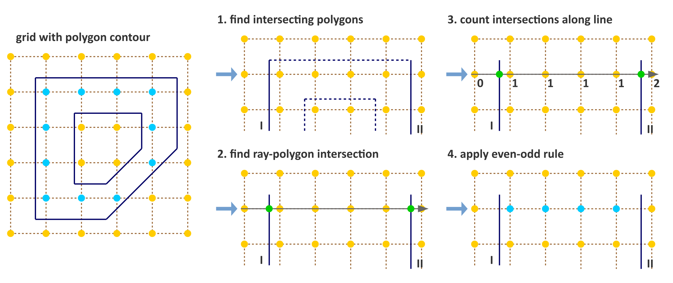
Fig. 2 Simple algorithm to determine which pixels are inside a 2D polygon. The suggested implementation consists of four steps: (1) Omit edges that will not intersect with the current row of voxel centers. (2) Calculate intersection points of edges I and II with the ray for the current row. (3) Determine the number of intersections crossed from ray origin to the row voxel centers. (4) Apply even-odd rule to determine whether voxel centers are inside the polygon.
Interpolation
VTM2
Texture feature sets require interpolation to isotropic voxel spacing to be rotationally invariant, and to allow comparison between image data from different samples, cohorts or batches. Voxel interpolation affects image feature values as many image features are sensitive to changes in voxel size [Yan2015][Bailly2016][Altazi2017][Shafiq-ul-Hassan2017][Shiri2017]. Maintaining consistent isotropic voxel spacing across different measurements and devices is therefore important for reproducibility. At the moment there are no clear indications whether upsampling or downsampling schemes are preferable. Consider, for example, an image stack of slices with \(1.0 \times 1.0 \times 3.0~\text{mm}^3\) voxel spacing. Upsampling to \(1.0 \times 1.0 \times 1.0~\text{mm}^3\) requires inference and introduces artificial information, while conversely downsampling to the largest dimension (\(3.0 \times 3.0 \times 3.0~\text{mm}^3\)) incurs information loss. Multiple-scaling strategies potentially offer a good trade-off [Vallieres2017]. Note that downsampling may introduce image aliasing artifacts. Downsampling may therefore require anti-aliasing filters prior to filtering [Mackin2017][Zwanenburg2018].
While in general 3D interpolation algorithms are used to interpolate 3D images, 2D interpolation within the image slice plane may be recommended in some situations. In 2D interpolation voxels are not interpolated between slices. This may be beneficial if, for example, the spacing between slices is large compared to the desired voxel size, and/or compared to the in-plane spacing. Applying 3D interpolation would either require inferencing a large number of voxels between slices (upsampling), or the loss of a large fraction of in-plane information (downsampling). The disadvantage of 2D interpolation is that voxel spacing is no longer isotropic, and as a consequence texture features can only be calculated in-plane.
Interpolation algorithms
Interpolation algorithms translate image intensities from the original image grid to an interpolation grid. In such grids, voxels are spatially represented by their center. Several algorithms are commonly used for interpolation, such as nearest neighbour, trilinear, tricubic convolution and tricubic spline interpolation. In short, nearest neighbour interpolation assigns the intensity of the most nearby voxel in the original grid to each voxel in the interpolation grid. Trilinear interpolation uses the intensities of the eight most nearby voxels in the original grid to calculate a new interpolated intensity using linear interpolation. Tricubic convolution and tricubic spline interpolation draw upon a larger neighbourhood to evaluate a smooth, continuous third-order polynomial at the voxel centers in the interpolation grid. The difference between tricubic convolution and tricubic spline interpolation lies in the implementation. Whereas tricubic spline interpolation evaluates the smooth and continuous third-order polynomial at every voxel center, tricubic convolution approximates the solution using a convolution filter. Though tricubic convolution is faster, with modern hardware and common image sizes, the difference in execution speed is practically meaningless. Both interpolation algorithms produce similar results, and both are often referred to as tricubic interpolation.
While no consensus exists concerning the optimal choice of interpolation algorithm, trilinear interpolation is usually seen as a conservative choice. It does not lead to the blockiness produced by nearest neighbour interpolation that introduces bias in local textures [Hatt2016]. Nor does it lead to out-of-range intensities which may occur due to overshoot with tricubic and higher order interpolations. The latter problem can occur in acute intensity transitions, where the local neighbourhood itself is not sufficiently smooth to evaluate the polynomial within the allowed range. Tricubic methods, however, may retain tissue contrast differences better. Particularly when upsampling, trilinear interpolation may act as a low-pass filter which suppresses higher spatial frequencies and cause artefacts in high-pass spatial filters. Interpolation algorithms and their advantages and disadvantages are treated in more detail elsewhere, e.g. [thevenaz2000image].
In a phantom study, [Larue2017] compared nearest neighbour, trilinear and tricubic interpolation and indicated that feature reproducibility is dependent on the selected interpolation algorithm, i.e. some features were more reproducible using one particular algorithm.
Rounding image intensities after interpolation
68QD
Image intensities may require rounding after interpolation, or the application of cut-off values. For example, in CT images intensities represent Hounsfield Units, and these do not take non-integer values. Following voxel interpolation, interpolated CT intensities are thus rounded to the nearest integer.
Partial volume effects in the ROI mask
E8H9
If the image on which the ROI mask was defined, is interpolated after the ROI was segmented, the ROI mask \(\mathbf{R}\) should likewise be interpolated to the same dimensions. Interpolation of the ROI mask is best conducted using either the nearest neighbour or trilinear interpolation methods, as these are guaranteed to produce meaningful masks. Trilinear interpolation of the ROI mask leads to partial volume effects, with some voxels containing fractions of the original voxels. Since a ROI mask is a binary mask, such fractions need to be binarised by setting a partial volume threshold \(\delta\):
A common choice for the partial volume threshold is \(\delta=0.5\). For nearest neighbour interpolation the ROI mask does not contain partial volume fractions, and may be used directly.
Interpolation results depend on the floating point representation used
for the image and ROI masks. Floating point representations should at
least be full precision (32-bit) to avoid rounding errors.
Interpolation grid
UMPJ
Interpolated voxel centers lie on the intersections of a regularly spaced grid. Grid intersections are represented by two coordinate systems. The first coordinate system is the grid coordinate system, with origin at \((0.0, 0.0, 0.0)\) and distance between directly neighbouring voxel centers (spacing) of \(1.0\). The grid coordinate system is the coordinate system typically used by computers, and consequentially, by interpolation algorithms. The second coordinate system is the world coordinate system, which is typically found in (medical) imaging and provides an image scale. As the desired isotropic spacing is commonly defined in world coordinate dimensions, conversions between world coordinates and grid coordinates are necessary, and are treated in more detail after assessing grid alignment methods.
Grid alignment affects feature values and is non-trivial. Three common grid alignments may be identified, and are shown in Fig. 3:
- Fit to original grid (58MB). In this case the interpolation grid is deformed so that the voxel centers at the grid intersections overlap with the original grid vertices. For an original \(4\times4\) voxel grid with spacing \((3.00, 3.00)\) mm and a desired interpolation spacing of \((2.00, 2.00)\) mm we first calculate the extent of the original voxel grid in world coordinates leading to an extent of \(((4-1)\,3.00, ((4-1)\,3.00) = (9.00, 9.00)\) mm. In this case the interpolated grid will not exactly fit the original grid. Therefore we try to find the closest fitting grid, which leads to a \(6\times 6\) grid by rounding up \((9.00/2.00, 9.00/2.00)\). The resulting grid has a grid spacing of \((1.80, 1.80)\) mm in world coordinates, which differs from the desired grid spacing of \((2.00, 2.00)\) mm.
- Align grid origins (SBKJ). A simple approach which conserves the desired grid spacing is the alignment of the origins of the interpolation and original grids. Keeping with the same example, the interpolation grid is \((6 \times 6)\). The resulting voxel grid has a grid spacing of \((2.00, 2.00)\) mm in world coordinates. By definition both grids are aligned at the origin, \((0.00, 0.00)\).
- Align grid centers (3WE3). The position of the origin may depend on image meta-data defining image orientation. Not all software implementations may process this meta-data the same way. An implementation-independent solution is to align both grids on the grid center. Again, keeping with the same example, the interpolation grid is \((6 \times 6)\). Thus, the resulting voxel grid has a grid spacing of \((2.00, 2.00)\) mm in world coordinates.
Align grid centers is recommended as it is implementation-independent and achieves the desired voxel spacing. Technical details of implementing align grid centers are described below.
Interpolation grid dimensions
026Q
The dimensions of the interpolation grid are determined as follows. Let \(n_a\) be the number of points along one axis of the original grid and \(s_{a,w}\) their spacing in world coordinates. Then, let \(s_{b,w}\) be the desired spacing after interpolation. The axial dimension of the interpolated mesh grid is then:
Rounding towards infinity guarantees that the interpolation grid exists even when the original grid contains few voxels. However, it also means that the interpolation mesh grid is partially located outside of the original grid. Extrapolation is thus required. Padding the original grid with the intensities at the boundary is recommended. Some implementations of interpolation algorithms may perform this padding internally.
Interpolation grid position
QCY4
For the align grid centers method, the positions of the interpolation grid points are determined as follows. As before, let \(n_a\) and \(n_b\) be the dimensions of one axis in the original and interpolation grid, respectively. Moreover, let \(s_{a,w}\) be the original spacing and \(s_{b,w}\) the desired spacing for the same axis in world coordinates. Then, with \(x_{a,w}\) the origin of the original grid in world coordinates, the origin of the interpolation grid is located at:
In the grid coordinate system, the original grid origin is located at \(x_{a,g} = 0\). The origin of the interpolation grid is then located at:
Here the fraction \(s_{b,w}/s_{a,w}= s_{b,g}\) is the desired spacing in grid coordinates. Thus, the interpolation grid points along the considered axis are located at grid coordinates:
Naturally, the above description applies to each grid axis.
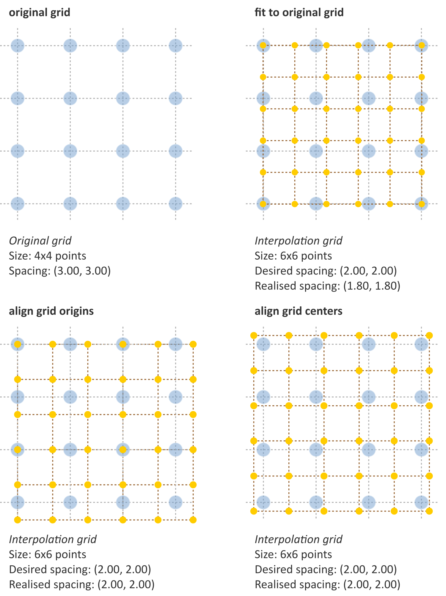
Fig. 3 Different interpolation mesh grids based on an original \(4\times 4\) grid with \((3.00, 3.00)\) mm spacing. The desired interpolation spacing is \((2.00, 2.00)\) mm. Fit to original grid creates an interpolation mesh grid that overlaps with the corners of the original grid. Align grid origins creates an interpolation mesh grid that is positioned at the origin of the original grid. Align grid centers creates an interpolation grid that is centered on the center of original and interpolation grids.
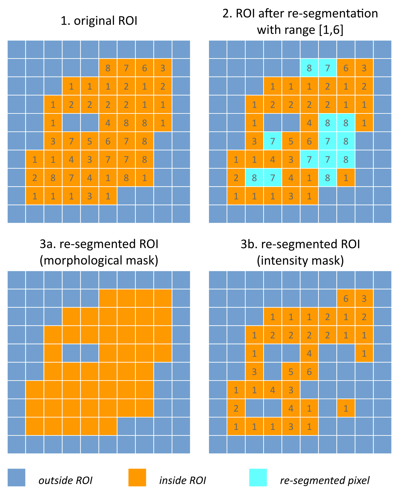
Fig. 4 Example showing how intensity and morphological masks may differ due to re-segmentation. (1) The original region of interest (ROI) is shown with pixel intensities. (2) Subsequently, the ROI is re-segmented to only contain values in the range \([1,6]\). Pixels outside this range are marked for removal from the intensity mask. (3a) Resulting morphological mask, which is identical to the original ROI. (3b) Re-segmented intensity mask. Note that due to re-segmentation, intensity and morphological masks are different.
Re-segmentation
IF9H
Re-segmentation entails updating the ROI mask \(\mathbf{R}\) based on corresponding voxel intensities \(\mathbf{X}_{gl}\). Re-segmentation may be performed to exclude voxels from a previously segmented ROI, and is performed after interpolation. An example use would be the exclusion of air or bone voxels from an ROI defined on CT imaging. Two common re-segmentation methods are described in this section. Combining multiple re-segmentation methods is possible. In this case, the intersection of the intensity ranges defined by the re-segmentation methods is used.
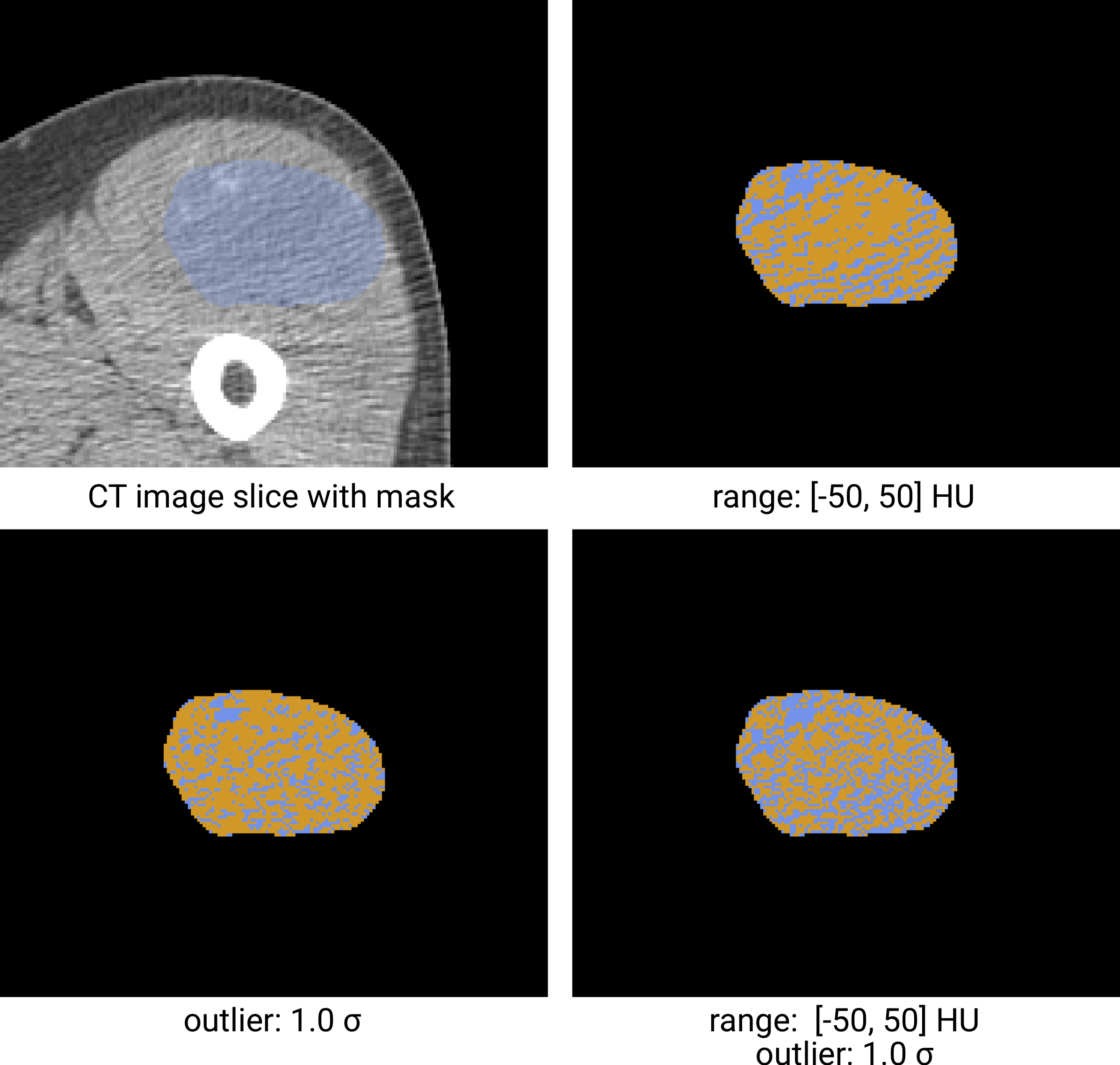
Fig. 5 Re-segmentation example based on a CT-image. The masked region (blue) is re-segmented to create an intensity mask (orange). Examples using three different re-segmentation parameter sets are shown. The bottom right combines the range and outlier re-segmentation, and the resulting mask is the intersection of the masks in the other two examples. Image data from Vallières et al. [Vallieres2015][Vallieres2015-hv][Clark2013].
Intensity and morphological masks of an ROI
ECJF
Conventionally, an ROI consists of a single mask. However, re-segmentation may lead to exclusion of internal voxels, or divide the ROI into sub-volumes. To avoid undue complexity by again updating the re-segmented ROI for a more plausible morphology, we define two separate ROI masks.
The morphological mask (G5KJ) is not re-segmented and maintains the original morphology as defined by an expert and/or (semi-)automatic segmentation algorithms.
The intensity mask (SEFI) can be re-segmented and will contain only the selected voxels. For many feature families, only this is important. However, for morphological and grey level distance zone matrix (GLDZM) feature families, both intensity and morphological masks are used. A two-dimensional schematic example is shown in Fig. 4, and a real example is shown in Fig. 5.
Range re-segmentation
USB3
Re-segmentation may be performed to remove voxels from the intensity mask that fall outside of a specified range. An example is the exclusion of voxels with Hounsfield Units indicating air and bone tissue in the tumour ROI within CT images, or low activity areas in PET images. Such ranges of intensities of included voxels are usually presented as a closed interval \(\left[ a,b\right]\) or half-open interval \(\left[a,\infty\right)\), respectively. For arbitrary intensity units (found in e.g. raw MRI data, uncalibrated microscopy images, and many spatial filters), no re-segmentation range can be provided.
When a re-segmentation range is defined by the user, it needs to be propagated and used for the calculation of features that require a specified intensity range (e.g. intensity-volume histogram features) and/or that employs fixed bin size discretisation. Recommendations for the possible combinations of different imaging intensity definitions, re-segmentation ranges and discretisation algorithms are provided in Table 1.
Intensity outlier filtering
7ACA
ROI voxels with outlier intensities may be removed from the intensity mask. One method for defining outliers was suggested by [Vallieres2015] after [Collewet2004]. The mean \(\mu\) and standard deviation \(\sigma\) of grey levels of voxels assigned to the ROI are calculated. Voxels outside the range \(\left[\mu - 3\sigma, \mu + 3\sigma\right]\) are subsequently excluded from the intensity mask.
ROI extraction
1OBP
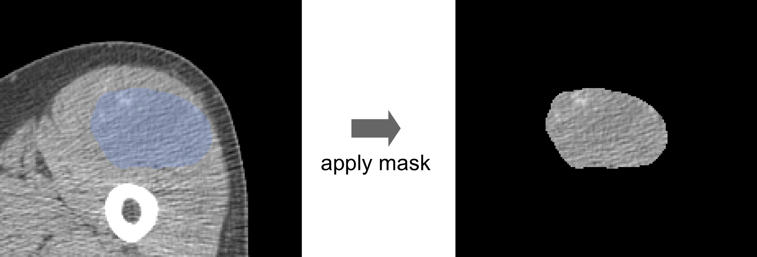
Fig. 6 Masking of an image by the ROI mask during ROI extraction. Intensities outside the ROI are excluded. Image data from Vallières et al. [Vallieres2015][Vallieres2015-hv][Clark2013].
Many feature families require that the ROI is isolated from the surrounding voxels. The ROI intensity mask is used to extract the image volume to be studied. Excluded voxels are commonly replaced by a placeholder value, often NaN. This placeholder value may then used to exclude these voxels from calculations. Voxels included in the ROI mask retain their original intensity. An example is shown in Fig. 6.
Intensity discretisation
4R0B
Discretisation or quantisation of image intensities inside the ROI is often required to make calculation of texture features tractable [Yip2016], and possesses noise-suppressing properties as well. An example of discretisation is shown in Fig. 7.
Two approaches to discretisation are commonly used. One involves the discretisation to a fixed number of bins, and the other discretisation with a fixed bin width. As we will observe, there is no inherent preference for one or the other method. However, both methods have particular characteristics (as described below) that may make them better suited for specific purposes. Note that the lowest bin always has value \(1\), and not \(0\). This ensures consistency for calculations of texture features, where for some features grey level \(0\) is not allowed.
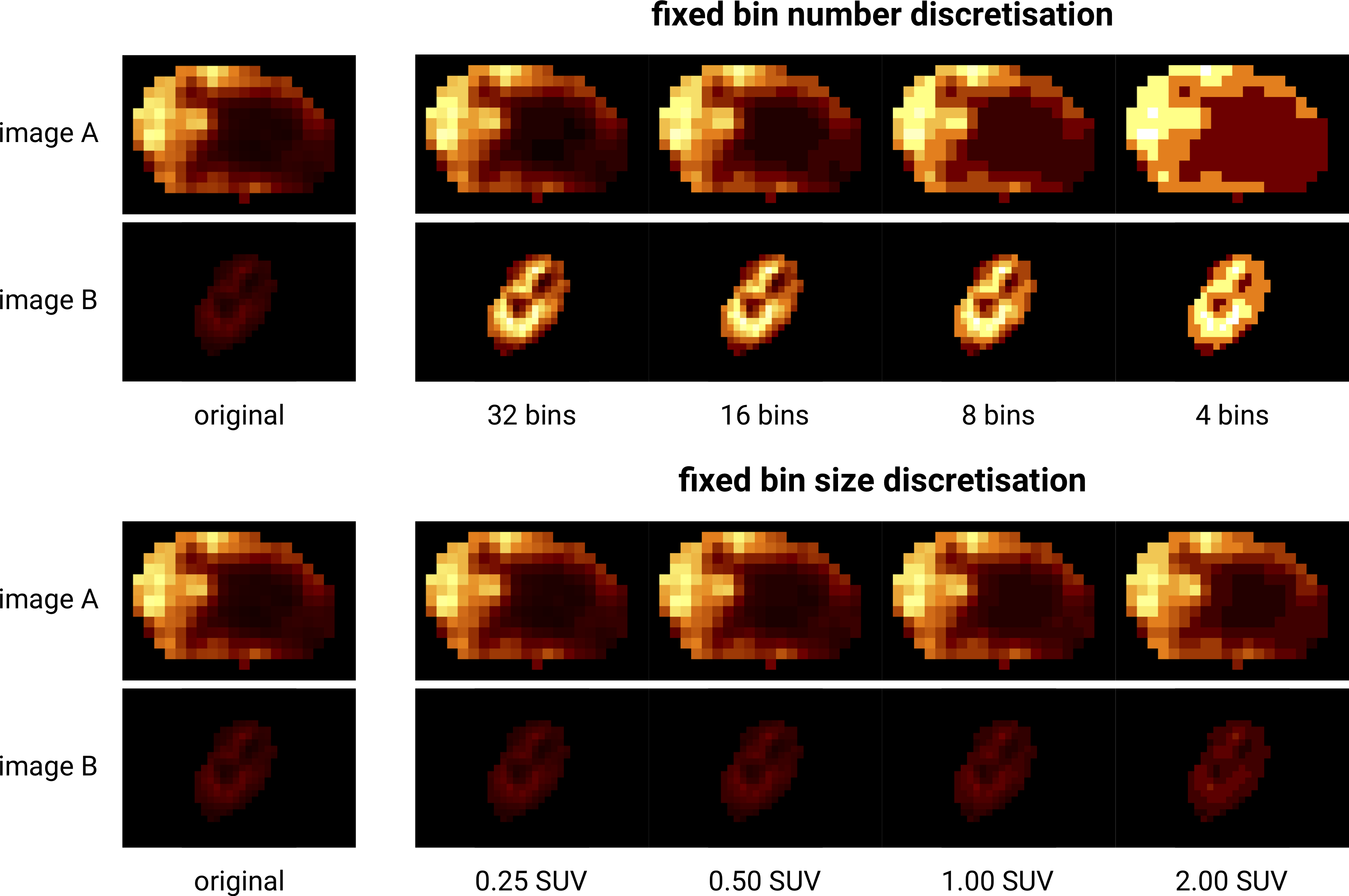
Fig. 7 Discretisation of two different 18F-FDG-PET images with SUVmax of \(27.8\) (A) and \(6.6\) (B). Fixed bin number discretisation adjust the contrast between the two images, with the number of bins determining the coarseness of the discretised image. Fixed bin size discretisation leaves the contrast differences between image A and B intact. Increasing the bin size increases the coarseness of the discretised image. Image data from Vallières et al. [Vallieres2015][Vallieres2015-hv][Clark2013].
Fixed bin number
K15C
In the fixed bin number method, intensities \(X_{gl}\) are discretised to a fixed number of \(N_g\) bins. It is defined as follows:
In short, the intensity \(X_{gl,k}\) of voxel \(k\) is corrected by the lowest occurring intensity \(X_{gl,min}\) in the ROI, divided by the bin width \(\left(X_{gl,max}-X_{gl,min}\right)/N_g\), and subsequently rounded down to the nearest integer (floor function).
The fixed bin number method breaks the relationship between image intensity and physiological meaning (if any). However, it introduces a normalising effect which may be beneficial when intensity units are arbitrary (e.g. raw MRI data and many spatial filters), and where contrast is considered important. Furthermore, as values of many features depend on the number of grey levels found within a given ROI, the use of a fixed bin number discretisation algorithm allows for a direct comparison of feature values across multiple analysed ROIs (e.g. across different samples).
Fixed bin size
Q3RU
Fixed bin size discretisation is conceptually simple. A new bin is assigned for every intensity interval with width \(w_b\); i.e. \(w_b\) is the bin width, starting at a minimum \(X_{gl,min}\). The minimum intensity may be a user-set value as defined by the lower bound of the re-segmentation range, or data-driven as defined by the minimum intensity in the ROI \(X_{gl,min}=\text{min} \left( X_{gl} \right)\). In all cases, the method used and/or set minimum value must be clearly reported. However, to maintain consistency between samples, we strongly recommend to always set the same minimum value for all samples as defined by the lower bound of the re-segmentation range (e.g. HU of -500 for CT, SUV of 0 for PET, etc.). In the case that no re-segmentation range may be defined due to arbitrary intensity units (e.g. raw MRI data and many spatial filters), the use of the fixed bin size discretisation algorithm is not recommended.
The fixed bin size method has the advantage of maintaining a direct relationship with the original intensity scale, which could be useful for functional imaging modalities such as PET.
Discretised intensities are computed as follows:
In short, the minimum intensity \(X_{gl,min}\) is subtracted from intensity \(X_{gl,k}\) in voxel \(k\), and then divided by the bin width \(w_b\). The resulting value is subsequently rounded down to the nearest integer (floor function), and \(1\) is added to arrive at the discretised intensity.
Other methods
Many other methods and variations for discretisation exist, but are not described in detail here. [Vallieres2015] described the use of intensity histogram equalisation and Lloyd-Max algorithms for discretisation. Intensity histogram equalisation involves redistributing intensities so that the resulting bins contain a similar number of voxels, i.e. contrast is increased by flattening the histogram as much as possible [Hall1971]. Histogram equalisation of the ROI imaging intensities can be performed before any other discretisation algorithm (e.g. FBN, FSB, etc.), and it also requires the definition of a given number of bins in the histogram to be equalised. The Lloyd-Max algorithm is an iterative clustering method that seeks to minimise mean squared discretisation errors [Max1960][Lloyd1982].
Recommendations
The discretisation method that leads to optimal feature inter- and intra-sample reproducibility is modality-dependent. Usage recommendations for the possible combinations of different imaging intensity definitions, re-segmentation ranges and discretisation algorithms are provided in Table 1. Overall, the discretisation choice has a substantial impact on intensity distributions, feature values and reproducibility [Hatt2015][Leijenaar2015a][vanVelden2016][Desseroit2017][Hatt2016][Shafiq-ul-Hassan2017][Altazi2017].
| Imaging intensity units\(^{(1)}\) | Re-segmentation range | FBN\(^{(2)}\) | FBS\(^{(3)}\) |
|---|---|---|---|
| \([a,b]\) | ✔ | ✔ | |
| calibrated | \([a,\infty)\) | ✔ | ✔ |
| none | ✔ | ✕ | |
| arbitrary | none | ✔ | ✕ |
Feature calculation
Feature calculation is the final processing step where feature descriptors are used to quantify characteristics of the ROI. After calculation such features may be used as image biomarkers by relating them to physiological and medical outcomes of interest. Feature calculation is handled in full details in the next chapter.
Let us recall that the image processing steps leading to image biomarker calculations can be performed in many different ways, notably in terms of spatial filtering, segmentation, interpolation and discretisation parameters. Furthermore, it is plausible that different texture features will better quantify the characteristics of the ROI when computed using different image processing parameters. For example, a lower number of grey levels in the discretisation process (e.g. 8 or 16) may allow to better characterize the sub-regions of the ROI using grey level size zone matrix (GLSZM) features, whereas grey level co-occurence matrix (GLCM) features may be better modeled with a higher number of grey levels (e.g. 32 or 64). Overall, these possible differences opens the door to the optimization of image processing parameters for each different feature in terms of a specific objective. For the specific case of the optimization of image interpolation and discretisation prior to texture analysis, Vallières et al. [Vallieres2015] have named this process texture optimization. The authors notably suggested that the texture optimization process could have significant influence of the prognostic capability of subsequent features. In another study [Vallieres2017], the authors constructed predictive models using textures calculated from all possible combinations of PET and CT images interpolated at four isotropic resolutions and discretised with two different algorithms and four numbers of grey levels.