Reference data sets
Reference values for features were obtained using a digital image phantom and the CT image of a lung cancer patient, which are described below. The same data sets can be used to verify radiomics software implementations. The data sets themselves may be found here: https://github.com/theibsi/data_sets.
Digital phantom
A small digital phantom was developed to derive image features manually and compare these values with values obtained from radiomics software implementations. The phantom is shown in Fig. 20. The phantom has the following characteristics:
- The phantom consists of \(5 \times 4 \times 4\) \((x,y,z)\) voxels.
- A slice consists of the voxels in \((x,y)\) plane for a particular slice at position \(z\). Slices are therefore stacked in the \(z\) direction.
- Voxels are \(2.0 \times 2.0 \times 2.0\) mm in size.
- Not all voxels are included in the region of interest. Several excluded voxels are located on the outside of the ROI, and one internal voxel was excluded as well. Voxels excluded from the ROI are shown in blue in Fig. 20.
- Some intensities are not present in the phantom. Notably, grey levels \(2\) and \(5\) are absent. \(1\) is the lowest grey level present in the ROI, and \(6\) the highest.
Computing image features
The digital phantom was designed to not require image processing prior to calculating the features. Thus, feature calculation is done directly on the phantom itself. The following should be taken into account for calculating image features:
- Discretisation is not required. All features are to be calculated using the phantom as it is. Alternatively, one could use a fixed bin size discretisation of 1 or fixed bin number discretisation of 6 bins, which does not alter the contents of the phantom.
- Grey level co-occurrence matrices are symmetrical and calculated for (Chebyshev) distance \(\delta=1\).
- Neighbouring grey level dependence and neighbourhood grey tone difference matrices are likewise calculated for (Chebyshev) distance \(\delta=1\). Additionally, the neighbouring grey level dependence coarseness parameter has the value \(\alpha=0\).
- Because discretisation is lacking, most intensity-based statistical features will match their intensity histogram-based analogues in value.
- The ROI morphological and intensity masks are identical for the digital phantom, due to lack of re-segmentation.
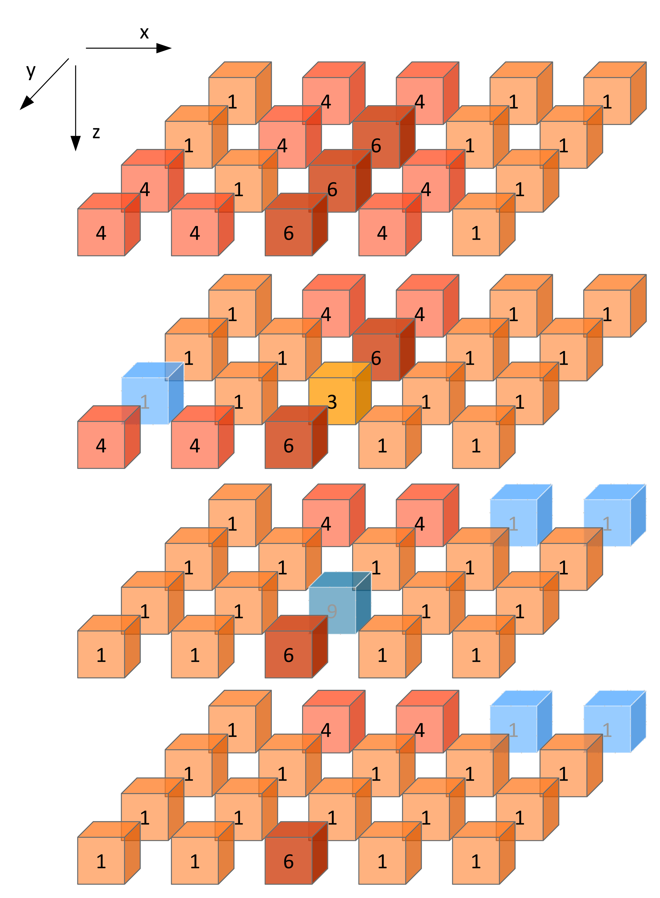
Fig. 20 Exploded view of the test volume. The number in each voxel corresponds with its grey level. Blue voxels are excluded from the region of interest. The coordinate system is so that \(x\) increases from left to right, \(y\) increases from back to front and \(z\) increases from top to bottom, as is indicated by the axis definition in the top-left.
Lung cancer CT image
A small data set of CT images from four non-small-cell lung carcinoma
patients was made publicly available to serve as radiomics phantoms
(DOI:10.17195/candat.2016.08.1).
We use the image for the first patient (PAT1) to obtain feature
reference values for different configurations of the image processing
scheme, as detailed below.
The CT image set is stored as a stack of slices in DICOM format. The
image slices can be identified by the DCM_IMG prefix. The gross
tumour volume (GTV) was delineated and is used as the region of interest
(ROI). Contour information is stored as an RT structure set in the DICOM
file starting with DCM_RS. For broader use, both the DICOM set
and segmentation mask have been converted to the NIfTI format. When
using the data in NIfTI format, both image stacks should be
converted to (at least) 32-bit floating point and rounded to the nearest
integer before further processing.
We defined five image processing configurations to test different image processing methods, see Configurations. While most settings are self-explanatory, there are several aspects that require some attention. Configurations are divided in 2D and 3D approaches. For the 2D configurations (A, B), image interpolation is conducted within the slice, and likewise texture features are extracted from the in-slice plane, and not volumetrically (3D). For the 3D configurations (C-E) interpolation is conducted in three dimensions, and features are likewise extracted volumetrically. Discretisation is moreover required for texture, intensity histogram and intensity-volume histogram features, and both fixed bin number and fixed bin size algorithms are tested.
Notes on interpolation
Interpolation has a major influence on feature values. Different implementations of the same interpolation method may ostensibly provide the same functionality, but may use different interpolation grids. It is therefore recommended to read the documentation of the particular implementation to assess if the implementation allows or implements the following:
- The spatial origin of the original (input) grid in world coordinates
matches the
DICOMorigin by definition. - The size of the interpolation grid is determined by rounding the fractional grid size towards infinity, i.e. a ceiling operation. This prevents the interpolation grid from disappearing for very small images, but is otherwise an arbitrary choice.
- The centers of the interpolation and original image grids should be aligned, i.e. the interpolation grid is centered on the center of the original image grid. This prevents spacing inconsistencies in the interpolation grid and avoids potential issues with grid orientation.
- The extent of the interpolation grid is, by definition, always equal or larger than that of the original grid. This means that intensities at the grid boundary are extrapolated. To facilitate this process, the image should be sufficiently padded with voxels that take on the nearest boundary intensity.
- The floating point representation of the image and the ROI masks
affects interpolation precision, and consequentially feature values.
Image and ROI masks should at least be represented at full precision
(
32-bit) to avoid rounding errors. One example is the unintended exclusion of voxels from the interpolated ROI mask, which occurs when interpolation yields 0.4999…instead of 0.5. When images and ROI masks are converted to full precision from lower precision (e.g.16-bit), values may require rounding if the original data were integer values, such as Hounsfield Units or the ROI mask labels.
More details are provided in the Interpolation section.
Diagnostic features
Identifying issues with an implementation of the image processing sequence may be challenging. Multiple steps follow one another and differences propagate. Hence we define a small number of diagnostic features that describe how the image and ROI masks change with each image processing step. These diagnostic features also have reference values that may be found in IBSI compliance check spreadsheet.
Initial image stack.
The following features may be used to describe the initial image stack (i.e. after loading image data for processing):
- Image dimensions. This describes the image dimensions in voxels along the different image axes.
- Voxel dimensions. This describes the voxel dimensions in mm. The dimension along the z-axis is equal to the distance between the origin voxels of two adjacent slices, and is generally equal to the slice thickness.
- Mean intensity. This is the average intensity within the entire image.
- Minimum intensity. This is the lowest intensity within the entire image.
- Maximum intensity. This is the highest intensity within the entire image.
Interpolated image stack.
The above features may also be used to describe the image stack after image interpolation.
Initial region of interest.
The following descriptors are used to describe the region of interest (ROI) directly after segmentation of the image:
- ROI intensity mask dimensions. This describes the dimensions, in voxels, of the ROI intensity mask.
- ROI intensity mask bounding box dimensions. This describes the dimensions, in voxels, of the bounding box of the ROI intensity mask.
- ROI morphological mask bounding box dimensions. This describes the dimensions, in voxels, of the bounding box of the ROI morphological mask.
- Number of voxels in the ROI intensity mask. This describes the number of voxels included in the ROI intensity mask.
- Number of voxels in the ROI morphological mask. This describes the number of voxels included in the ROI intensity mask.
- Mean ROI intensity. This is the mean intensity of image voxels within the ROI intensity mask.
- Minimum ROI intensity. This is the lowest intensity of image voxels within the ROI intensity mask.
- Maximum ROI intensity. This is the highest intensity of image voxels within the ROI intensity mask.
Interpolated region of interest.
The same features can be used to describe the ROI after interpolation of the ROI mask.
Re-segmented region of interest.
Again, the same features as above can be used to describe the ROI after re-segmentation.
Computing image features
Unlike the digital phantom, the lung cancer CT image does require additional image processing, which is done according to the processing configurations described in the tables below. The following should be taken into account when calculating image features:
- Grey level co-occurrence matrices are symmetrical and calculated for (Chebyshev) distance \(\delta=1\).
- Neighbouring grey level dependence and neighbourhood grey tone difference matrices are likewise calculated for (Chebyshev) distance \(\delta=1\). Additionally, the neighbouring grey level dependence coarseness parameter \(\alpha=0\).
- Intensity-based statistical features and their intensity histogram-based analogues will differ in value due to discretisation, in contrast to the same features for the digital phantom.
- Due to re-segmentation, the ROI morphological and intensity masks are not identical.
- Calculation of IVH feature: since by default CT contains calibrated and discrete intensities, no separate discretisation prior to the calculation of intensity-volume histogram features is required. This is the case for configurations A, B and D (i.e. “calibrated intensity units – discrete case”). However, for configurations C and E, we re-discretise the ROI intensities prior to calculation of intensity-volume histogram features to allow for testing of of these methods. Configuration C simulates the “calibrated intensity units – continuous case”, while configuration E simulates the “arbitrary intensity units” case where the re-segmentation range is not used. For details, please consult the Intensity-volume histogram features section.
Configurations
Below are tables for the different configurations for image processing of the lung cancer CT Phantom. For details, refer to the corresponding sections in chapter Image processing.
Configuration A
| Parameter | Config A | |
|---|---|---|
| sample identifier | PAT1 | |
| ROI name | GTV-1 | |
| slice-wise or single volume (3D) | 2D | |
| interpolation | no | |
| resampled voxel spacing (mm) | – | |
| interpolation method | – | |
| intensity rounding | – | |
| ROI interpolation method | – | |
| ROI partial mask volume | – | |
| re-segmentation | ||
| range (HU) | [−500, 400] | |
| outlier filtering | no | |
| discretisation | ||
| texture and IH | FBS: 25HU | |
| IVH | no | |
| texture parameters | ||
| GLCM, NGTDM, NGLDM distance | 1 | |
| GLSZM, GLDZM linkage distance | 1 | |
| NGLDM coarseness | 0 |
Configuration B
| Parameter | Config B | |
|---|---|---|
| sample identifier | PAT1 | |
| ROI name | GTV-1 | |
| slice-wise or single volume (3D) | 2D | |
| interpolation | yes | |
| resampled voxel spacing (mm) | 2 × 2 (axial) | |
| interpolation method | bilinear | |
| intensity rounding | nearest integer | |
| ROI interpolation method | bilinear | |
| ROI partial mask volume | 0.5 | |
| re-segmentation | ||
| range (HU) | [−500, 400] | |
| outlier filtering | no | |
| discretisation | ||
| texture and IH | FBN: 32 bins | |
| IVH | no | |
| texture parameters | ||
| GLCM, NGTDM, NGLDM distance | 1 | |
| GLSZM, GLDZM linkage distance | 1 | |
| NGLDM coarseness | 0 |
Configuration C
| Parameter | Config C | |
|---|---|---|
| sample identifier | PAT1 | |
| ROI name | GTV-1 | |
| slice-wise or single volume (3D) | 3D | |
| interpolation | yes | |
| resampled voxel spacing (mm) | 2 × 2× 2 | |
| interpolation method | trilinear | |
| intensity rounding | nearest integer | |
| ROI interpolation method | trilinear | |
| ROI partial mask volume | 0.5 | |
| re-segmentation | ||
| range (HU) | [−1000, 400] | |
| outlier filtering | no | |
| discretisation | ||
| texture and IH | FBS: 25 HU | |
| IVH | FBS: 2.5 HU | |
| texture parameters | ||
| GLCM, NGTDM, NGLDM distance | 1 | |
| GLSZM, GLDZM linkage distance | 1 | |
| NGLDM coarseness | 0 |
Configuration D
| Parameter | Config D | |
|---|---|---|
| sample identifier | PAT1 | |
| ROI name | GTV-1 | |
| slice-wise or single volume (3D) | 3D | |
| interpolation | yes | |
| resampled voxel spacing (mm) | 2 × 2× 2 | |
| interpolation method | trilinear | |
| intensity rounding | nearest integer | |
| ROI interpolation method | trilinear | |
| ROI partial mask volume | 0.5 | |
| re-segmentation | ||
| range (HU) | no | |
| outlier filtering | 3σ | |
| discretisation | ||
| texture and IH | FBN: 32 bins | |
| IVH | no | |
| texture parameters | ||
| GLCM, NGTDM, NGLDM distance | 1 | |
| GLSZM, GLDZM linkage distance | 1 | |
| NGLDM coarseness | 0 |
Configuration E
| Parameter | Config E | |
|---|---|---|
| sample identifier | PAT1 | |
| ROI name | GTV-1 | |
| slice-wise or single volume (3D) | 3D | |
| interpolation | yes | |
| resampled voxel spacing (mm) | 2 × 2× 2 | |
| interpolation method | tricubic spline | |
| intensity rounding | nearest integer | |
| ROI interpolation method | trilinear | |
| ROI partial mask volume | 0.5 | |
| re-segmentation | ||
| range (HU) | [-1000,400] | |
| outlier filtering | 3σ | |
| discretisation | ||
| texture and IH | FBN: 32 bins | |
| IVH | 1000 bins | |
| texture parameters | ||
| GLCM, NGTDM, NGLDM distance | 1 | |
| GLSZM, GLDZM linkage distance | 1 | |
| NGLDM coarseness | 0 |
ROI: region of interest; HU: Hounsfield Unit; IH: intensity histogram; FBS: fixed bin size; FBN: fixed bin number; IVH: intensity-volume histogram; GLCM: grey level co-occurrence matrix; NGTDM: neighborhood grey tone difference matrix; NGLDM: neighbouring grey level dependence matrix; GLSZM: grey level size zone matrix; GLDZM: grey level distance zone matrix.